
| StartDate | EndDate | Status | Progress | Duration (in seconds) | Finished | RecordedDate | ResponseId | DistributionChannel | UserLanguage | socialmedia | gender | siblings | smed.hrs | gram.followers | fbfriends | tiktokFollow | eatatklein | kleinsatisfy | tvhours | countries | firstname | haircolor | belief.in.god | liveoncampus | numclasses | hs_students | firstjobage | covidtimes | eatmeat | operas | cigarettes | like.dance | shakespeare | voting | majordiv | hrs.sleep | height.unvalidated | shootingdrills | handedness |
|---|---|---|---|---|---|---|---|---|---|---|---|---|---|---|---|---|---|---|---|---|---|---|---|---|---|---|---|---|---|---|---|---|---|---|---|---|---|---|---|
| 2025-09-03 10:24:34 | 2025-09-03 10:52:58 | 0 | 100 | 1704 | 1 | 2025-09-03 10:52:58 | R_5YrnxZKSOlDoK4F | anonymous | EN | 14 | Male | 2 | 2 | 465 | NA | 18745 | 14 | 60 | 2 | 4 | 4 | 2 | 3 | 1 | 5 | 120 | 13 | 4 | 1 | 1 | 2 | 21 | 8 | 1 | 3 | 7 | 65 | 1 | 4 |
| 2025-09-03 13:23:05 | 2025-09-03 13:27:44 | 0 | 100 | 278 | 1 | 2025-09-03 13:27:44 | R_3ds3cgnFxWJow6v | anonymous | EN | 142 | female | 1 | 7 | 670 | 3 | 165 | 10 | 87 | 8 | 2 | 7 | 1 | 2 | 1 | 4 | 300 | 14 | 2 | 1 | 1 | 2 | 19 | 5 | 1 | 1 | 6 | 67 | 1 | 4 |
| 2025-09-03 13:22:21 | 2025-09-03 13:27:45 | 0 | 100 | 324 | 1 | 2025-09-03 13:27:45 | R_6WxUnBFzUvsqS0F | anonymous | EN | 14 | Female | 1 | 4 | 493 | NA | 714 | 10 | 40 | 6 | 4 | 6 | 2 | 3 | 1 | 4 | 500 | 16 | 0 | 2 | 0 | 1 | 19 | 4 | 1 | 3 | 8 | 66 | 1 | 4 |
| 2025-09-03 10:24:05 | 2025-09-03 14:43:30 | 0 | 100 | 15565 | 1 | 2025-09-03 14:43:30 | R_3zvh2m46usdvEcN | anonymous | EN | 142 | Female | 0 | 8 | 1718 | 592 | 184 | 4 | 25 | 4 | 3 | 6 | 1 | 1 | 1 | 4 | 400 | 16 | 1 | 1 | 0 | 2 | 18 | 4 | 1 | 3 | 8 | 68 | 1 | 5 |
| 2025-09-03 10:24:25 | 2025-09-03 15:10:30 | 0 | 100 | 17164 | 1 | 2025-09-03 15:10:30 | R_1Flk5XONhu4bLnP | anonymous | EN | 142 | woman | 2 | 4 | 1239 | 28 | 414 | 9 | 40 | 1 | 10 | 7 | 1 | 3 | 1 | 5 | 700 | 17 | 3 | 1 | 1 | 2 | 18 | 6 | 1 | 3 | 7 | 65 | 2 | 5 |
| 2025-09-03 15:15:30 | 2025-09-03 15:22:00 | 0 | 100 | 389 | 1 | 2025-09-03 15:22:01 | R_1qjANJnUMXRqoTQ | anonymous | EN | 14 | Female | 1 | 2 | 613 | NA | 1 | 14 | 90 | 2 | 2 | 6 | 1 | 3 | 1 | 4 | 2500 | 15 | 1 | 1 | 0 | 2 | 15 | 3 | 1 | 3 | 7 | 68 | 1 | 5 |
Today’s lab is focused on these objectives:
- Learning how to implement a basic hypothesis test in Jamovi
- Practicing some simple data visualization skills; we’ll do more next lab
- Understanding how z-tests for a single sample work
You’ll turn in an “answer sheet” on Brightspace. Please be sure to turn that in by next lab.
In today’s lab, we’re using data from a small sample and pretending it’s from a population. That’s fine, because we’re learning here—but in the future, you should not normally use a z-test to run analyses.
Although you will soon learn about hypothesis testing with means of samples, we’re going to talk about the hypothesis test when it pertains to an individual score today.
Data
You might want to start by downloading the data. The original (unedited) friends dataset is available on Brightspace, here.
We’ll eventually used a cleaned-up version, but not today.
Friends data
Before we do anything else, let’s talk about the data from your class (and a few friends). Here’s what some of the data look like (note that you can scroll to the right, but I have not printed all of the data here):
Many of you have collected data in Qualtrics before; this is what the data from Qualtrics look like. What you’ll see now is that it isn’t immediately usable.
Go ahead and open the friends-unedited.csv data in Jamovi. (If you didn’t download it before, it’s available under data above.) I haven’t edited any of these data yet. Explore the data a bit.
Check to make sure that your data has the values you’d expect. How many rows does it have? You’ll note that the first two rows (when this has been loaded into Jamovi) are extra information. Delete them. How many rows are left? (You can just scroll to the bottom.) Enter this value on Brightspace as #1 on your answer sheet.
Because these data were imported with text at the top, Jamovi doesn’t automatically know that some are numbers. (So almost all are categorical at the moment. Some it has designated as ID variables, and there is a real ID variable, here
ResponseId. Later, we’ll use the a cleaned-up version which doesn’t have this problem.) You’ll have to tell Jamovi when something is a number. Pick two variables you think should be Continuous (numeric). Under the Data or Variables tabs in the Ribbon, switch that variable to be continuous (or, possibly, ordinal).If we want to create a new variable that’s a rough combination of number of instagram followers with number of hours spent on social media, we might create it as a new variable where we divide the first (
gram.followers) by the second (smed.hrs). First, make sure Jamovi “knows” that both of those are continuous variables. Then, under the Data menu, use the Compute button to do this. Call the new variable something likesocial.quotient. (Remember that you can use the/for division.)
I’m not sure how to compute this new variable (expand for more)
You can read about computing variables here. In brief, you’ll click “Compute” under the Data tab, or insert a computed variable. Then, you’ll name it (social.quotient) and set its formula equal to the divided output of gram.followers / smed.hrs.
If those two variables haven’t been set to be continuous, this will not work! It will just be blank.
Find the range of how many students went to our respondents’ high schools (
hs_students). You will probably need to make this continuous, too, and then use Analyses -> Exploration -> Descriptives. Enter it as answer #2.How many different answers are there for gender are in these data? For the moment, just answer “from a computer’s perspective” (i.e., what the program is telling you, not how you understand it—and yes, an extra space means that the computer “sees”
Femaleas different fromFemale). Add this as answer #3 From a human’s perspective: well, it depends a bit on how you categorize them, right? There are some automated ways of dealing with this, but not (unfortunately) ones I know of in Jamovi or Excel/Sheets. Take some time to recode, and put everything in lower case—not in Levels but in the data directly, or in a new variable calledgender_recoded. (You can also do a “transform” as described here, which works well but requires playing around. If you’re feeling comfortable with this stuff, give it a try or come back to it later.) Do you put “woman” and “female” together? I imagine so. However, we actually have a nice set of responses that make this tricky, so make your own decisions at this point—I recommend going for five or fewer categories. (This is where some subjectivity comes into data analysis. We may briefly discuss how one should collect and report gender data; I have many thoughts. You can also read more about reporting gender from the APA, here. They give examples of how you might group folks in our sample.)Now go back to Analysis -> Exploration -> Descriptives. Put one of your numeric variables in Variables, and put the cleaned up Gender variable in the Split by box. Turn on a box plot, and check the checkbox to add the Data onto it. Your plot shouldn’t have any more than 5 boxes (because you narrowed down the gender categories.) Submit this plot as #4. (You can right click on the image and click “export” or copy, or you can take a screenshot from your computer. You may not use your phone to take a photograph of the computer screen.)
Friends questions
Now, we’ll use these friends data for a few simple questions.
- Would someone who was 6’5” be considered to have a “significantly different” height among Bard students?
- Would someone who doesn’t watch any TV be considered statistically-significantly different from other Bard students?
Steps of hypothesis-testing
Step 1
Step 1: Restate question as a research and null hypothesis
We asked: Would someone who was 6’5” be considered to have a “significantly different” height among Bard students? Read the questions below. I’ve answered them for you—you should click the question to see the answer.
What is the framing of this for the research hypothesis?
People who are as tall as this person are different from Bard students as a whole
What is the framing of this for the null hypothesis? (click to expand)
People who are as tall as this person are no different from Bard students as a whole
Ultimately, we’re interested in means, as you’ll remember—the statistical framing of these hypotheses. How do the means of people like this person compare to the means of students at Bard. We can frame the research hypothesis as: \(\mu_{\mathrm{Bard~students~of~this~height}}\neq\mu_{\mathrm{Bard~students~in~general}}\) and the null hypothesis as: \(\mu_{\mathrm{Bard~students~of~this~height}}=\mu_{\mathrm{Bard~students~in~general}}\)
Step 2
Step 2: Determine the characteristics of the comparison distribution
In this case, we’re continuing to use the distribution of z-scores. We’re moving into territory we didn’t get to in class, but we’ll return to it soon in class and you should feel free to ask questions here in lab.
Which of the following is/are true about a z-score distribution?
- We assume that it is normally-distributed
- It has a mean of 0
- It has a standard deviation of 1
- It is symmetrical
See the answer (click to expand)
They are all true. The z distribution is essentially a normal distribution with known characteristics of \(M=0\) and \(SD=1\). All normal distributions are by nature symmetrical.
Step 3
Step 3: Determine the sample cutoff score to reject the null hypothesis
We determine the cut-off score as the score that would be “as extreme” as to be hitting the p < .05 threshold. For a z-test, our cut-off score is going to be \(\pm{}1.96\). Let’s discuss how we get that.
What we actually want to get is the most extreme 5% of scores. These are going to be, from the center (mean) of the distribution, the bottom 2.5% of scores and the top 2.5% of scores. Something like this:
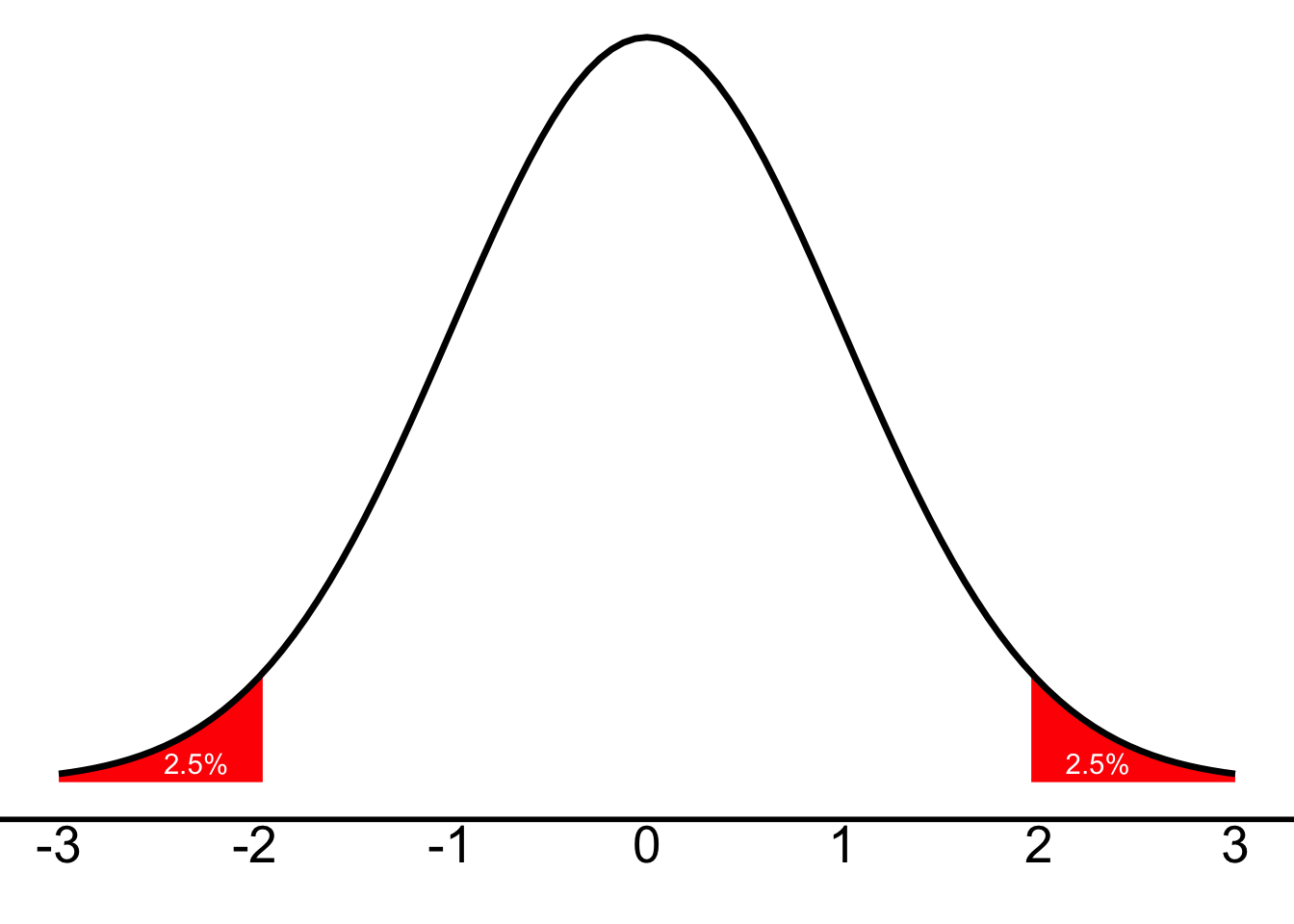
We can also think of those as cut-offs for the lowest 2.5% of scores and the highest 2.5% of scores. So the bottom 2.5% will be on the left, and the top-most 2.5% on the right—with 97.5% of scores below it.
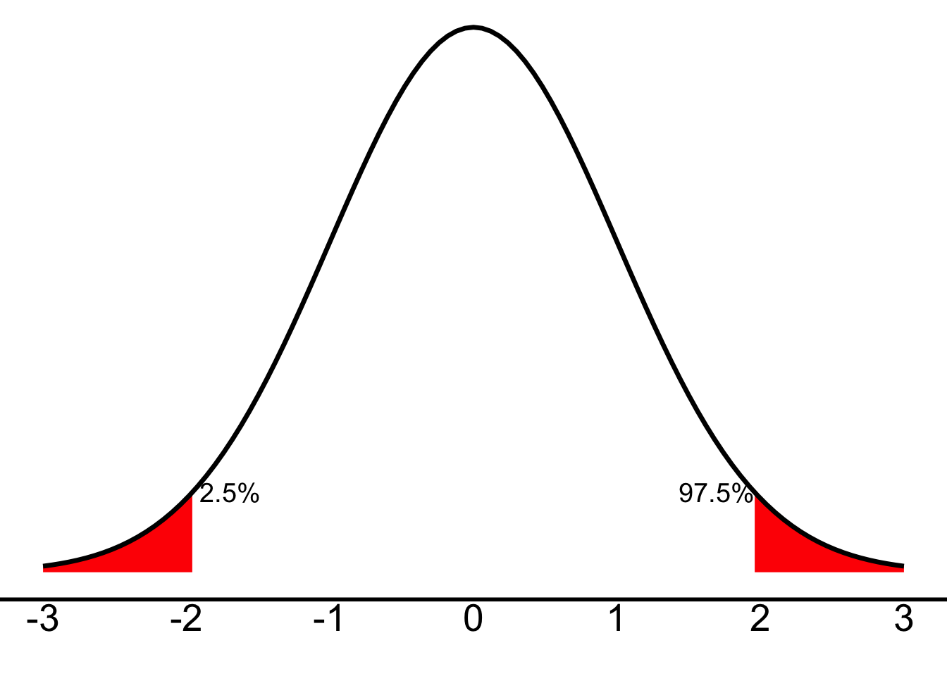
That is to say: if there’s 2.5% in each tail, then on the left side, 2.5% of scores are in that left, red tail. On the right side, 97.5% of scores will be to the left of the right, red tail.
Let’s look at a z-table. (Note that while the table later eventually skips to infinity, noted as Inf, in this one I intentionally ended so that your answer should be on the last page.) Click “next” until the “% in Tail” column on the right reads 2.50. What number (for z) represents 2.50% in the tail?
What number (for z) represents 2.50% in the tail? (click to expand)
It’s 1.96. Specifically, it’s \(\pm{}1.96\) – -1.96 below the mean on the left and +1.96 above the mean on the right.
Okay! With those two questions, we’ve gotten through Steps 2 and 3 for the first research question!
Step 4: Determine your sample’s score
The information on heights is saved in the data.
Find the range and mean of the variable height.unvalidated. If you’ve loaded it correctly, you should see the mean as 66.6 and the range as 5.11, 165 or (as max minus min) 159.89 (Jamovi seems to round to 160). You might note that the range doesn’t make much sense. I’ll tell you why: we asked for height, in inches, but someone seems to have given height in feet. That’s why the variable is called “unvalidated”; in Qualtrics we could have thrown an error there, but we chose not to. (Someone else probably gave their height in centimeters… thanks to them for adding some complications!)
You could also have caught this if you make a box plot:
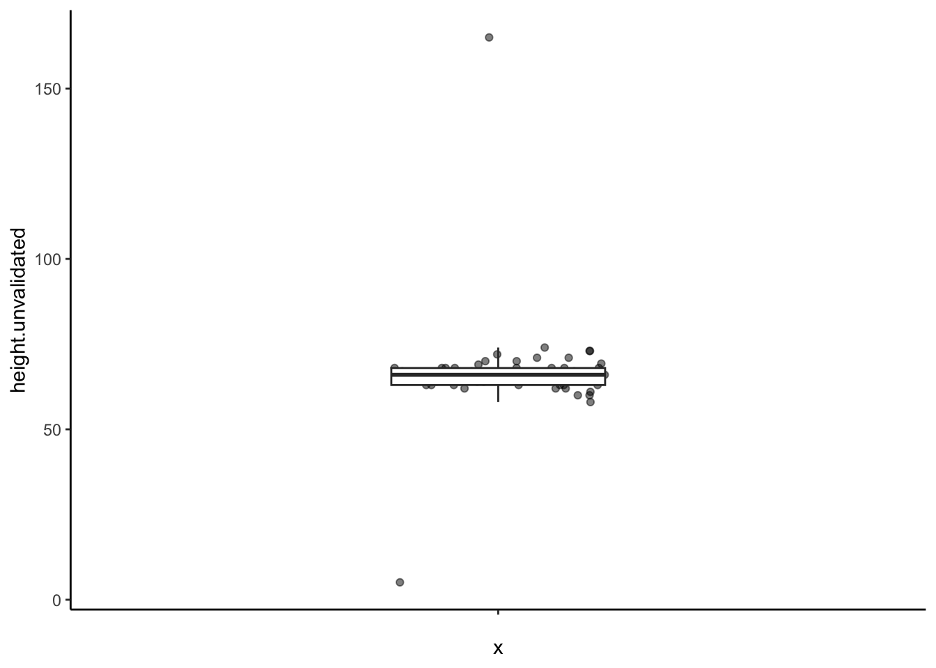
Find the one person who gave their height in feet, and (manually, probably) correct them to be in inches. Remember, 1 foot = 12 inches. In my mind, this person’s height is not 5.11 but is \(5'11''\); so that would be five feet and eleven inches.
But there’s also no way that someone is 165 inches tall! We have two choices here: remove this participant or assume that they answered with the height in centimeters. I’d suggest you assume the latter. Correct this person’s answer as well, assuming that there are 2.54 cm in 1 in. (You can round to 2 decimals.) In looking it over, you may also find this weird case where someone had their height as 69.29… I guess we leave it, but that’s a weird amount of precision!
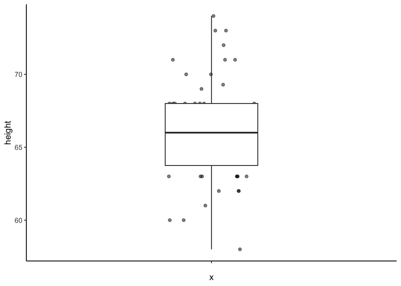
After fixing these data, find the mean, range, and standard deviation of height. This is question #5 on your answer sheet.
Your boxplot should look better now:
Let’s move on.
We now need to complete Step 4 and determine the z-score. We know how to determine a z-score already. Let’s do it. Remember that \(z=\frac{X-M}{SD}\) or (in population terms) \(z=\frac{X-\mu}{\sigma}\). So our sample—from which we’ll estimate the mean and standard deviation—will be students in this survey. You’ll see soon enough that we normally make additional corrections for the fact that this is only an estimate… but for today, let’s just make use of the means and standard deviations of the height in Jamovi. You should have gotten those in the same step where you found the range and mean. (Go find them if needed.)
Our research question is this: Would someone who was 6’5” be considered to have a “significantly different” height among Bard students? Well, now we can get the z-score for that person. Convert 6’5” to inches. Since \(z=(X-M)/SD\), we can fill this in from what we have. Solve for z; I recommend just doing it on paper. This is answer #6.
Step 5: Decide whether or not to reject the null hypothesis
Just by looking at your z-score, you should have an idea of whether or not we’ll reject the null. As we discussed in Steps 2 and 3, our cut-off is \(\pm1.96\).
Based on the z-score and the cutoff above, should we reject the null hypothesis?
Yes, because the z-score is higher than our cutoff. We can reject the null hypothesis—that there is no difference between this score and the population.
We can simply compare this score to our cutoff—is it more than \(+1.96\) or less than \(-1.96\)? It is larger than 1.96.
In this case, it’s actually a lot bigger. 99.92% of scores should be lower than this one. Having a height of 6’5” in our sample would be extremely unlikely—such a person would fall in the top 99.92% of the sample.
Compare to a z-table (where we would need to add 50% to the “% Mean to z” column or subtract the “% in Tail” column from 100%). Scroll down to get to the z we’ve found. (And scroll all the way down to see us eventually skip to infinity after we’re almost to the end of the tail.)
| z | % Mean to z | % in Tail |
|---|---|---|
| 0.00 | 0.00 | 50.00 |
| 0.01 | 0.40 | 49.60 |
| 0.02 | 0.80 | 49.20 |
| 0.03 | 1.20 | 48.80 |
| 0.04 | 1.60 | 48.40 |
| 0.05 | 1.99 | 48.01 |
| 0.06 | 2.39 | 47.61 |
| 0.07 | 2.79 | 47.21 |
| 0.08 | 3.19 | 46.81 |
| 0.09 | 3.59 | 46.41 |
| 0.10 | 3.98 | 46.02 |
| 0.11 | 4.38 | 45.62 |
| 0.12 | 4.78 | 45.22 |
| 0.13 | 5.17 | 44.83 |
| 0.14 | 5.57 | 44.43 |
| 0.15 | 5.96 | 44.04 |
| 0.16 | 6.36 | 43.64 |
| 0.17 | 6.75 | 43.25 |
| 0.18 | 7.14 | 42.86 |
| 0.19 | 7.53 | 42.47 |
| 0.20 | 7.93 | 42.07 |
| 0.21 | 8.32 | 41.68 |
| 0.22 | 8.71 | 41.29 |
| 0.23 | 9.10 | 40.90 |
| 0.24 | 9.48 | 40.52 |
| 0.25 | 9.87 | 40.13 |
| 0.26 | 10.26 | 39.74 |
| 0.27 | 10.64 | 39.36 |
| 0.28 | 11.03 | 38.97 |
| 0.29 | 11.41 | 38.59 |
| 0.30 | 11.79 | 38.21 |
| 0.31 | 12.17 | 37.83 |
| 0.32 | 12.55 | 37.45 |
| 0.33 | 12.93 | 37.07 |
| 0.34 | 13.31 | 36.69 |
| 0.35 | 13.68 | 36.32 |
| 0.36 | 14.06 | 35.94 |
| 0.37 | 14.43 | 35.57 |
| 0.38 | 14.80 | 35.20 |
| 0.39 | 15.17 | 34.83 |
| 0.40 | 15.54 | 34.46 |
| 0.41 | 15.91 | 34.09 |
| 0.42 | 16.28 | 33.72 |
| 0.43 | 16.64 | 33.36 |
| 0.44 | 17.00 | 33.00 |
| 0.45 | 17.36 | 32.64 |
| 0.46 | 17.72 | 32.28 |
| 0.47 | 18.08 | 31.92 |
| 0.48 | 18.44 | 31.56 |
| 0.49 | 18.79 | 31.21 |
| 0.50 | 19.15 | 30.85 |
| 0.51 | 19.50 | 30.50 |
| 0.52 | 19.85 | 30.15 |
| 0.53 | 20.19 | 29.81 |
| 0.54 | 20.54 | 29.46 |
| 0.55 | 20.88 | 29.12 |
| 0.56 | 21.23 | 28.77 |
| 0.57 | 21.57 | 28.43 |
| 0.58 | 21.90 | 28.10 |
| 0.59 | 22.24 | 27.76 |
| 0.60 | 22.57 | 27.43 |
| 0.61 | 22.91 | 27.09 |
| 0.62 | 23.24 | 26.76 |
| 0.63 | 23.57 | 26.43 |
| 0.64 | 23.89 | 26.11 |
| 0.65 | 24.22 | 25.78 |
| 0.66 | 24.54 | 25.46 |
| 0.67 | 24.86 | 25.14 |
| 0.68 | 25.17 | 24.83 |
| 0.69 | 25.49 | 24.51 |
| 0.70 | 25.80 | 24.20 |
| 0.71 | 26.11 | 23.89 |
| 0.72 | 26.42 | 23.58 |
| 0.73 | 26.73 | 23.27 |
| 0.74 | 27.04 | 22.96 |
| 0.75 | 27.34 | 22.66 |
| 0.76 | 27.64 | 22.36 |
| 0.77 | 27.94 | 22.06 |
| 0.78 | 28.23 | 21.77 |
| 0.79 | 28.52 | 21.48 |
| 0.80 | 28.81 | 21.19 |
| 0.81 | 29.10 | 20.90 |
| 0.82 | 29.39 | 20.61 |
| 0.83 | 29.67 | 20.33 |
| 0.84 | 29.95 | 20.05 |
| 0.85 | 30.23 | 19.77 |
| 0.86 | 30.51 | 19.49 |
| 0.87 | 30.78 | 19.22 |
| 0.88 | 31.06 | 18.94 |
| 0.89 | 31.33 | 18.67 |
| 0.90 | 31.59 | 18.41 |
| 0.91 | 31.86 | 18.14 |
| 0.92 | 32.12 | 17.88 |
| 0.93 | 32.38 | 17.62 |
| 0.94 | 32.64 | 17.36 |
| 0.95 | 32.89 | 17.11 |
| 0.96 | 33.15 | 16.85 |
| 0.97 | 33.40 | 16.60 |
| 0.98 | 33.65 | 16.35 |
| 0.99 | 33.89 | 16.11 |
| 1.00 | 34.13 | 15.87 |
| 1.01 | 34.38 | 15.62 |
| 1.02 | 34.61 | 15.39 |
| 1.03 | 34.85 | 15.15 |
| 1.04 | 35.08 | 14.92 |
| 1.05 | 35.31 | 14.69 |
| 1.06 | 35.54 | 14.46 |
| 1.07 | 35.77 | 14.23 |
| 1.08 | 35.99 | 14.01 |
| 1.09 | 36.21 | 13.79 |
| 1.10 | 36.43 | 13.57 |
| 1.11 | 36.65 | 13.35 |
| 1.12 | 36.86 | 13.14 |
| 1.13 | 37.08 | 12.92 |
| 1.14 | 37.29 | 12.71 |
| 1.15 | 37.49 | 12.51 |
| 1.16 | 37.70 | 12.30 |
| 1.17 | 37.90 | 12.10 |
| 1.18 | 38.10 | 11.90 |
| 1.19 | 38.30 | 11.70 |
| 1.20 | 38.49 | 11.51 |
| 1.21 | 38.69 | 11.31 |
| 1.22 | 38.88 | 11.12 |
| 1.23 | 39.07 | 10.93 |
| 1.24 | 39.25 | 10.75 |
| 1.25 | 39.44 | 10.56 |
| 1.26 | 39.62 | 10.38 |
| 1.27 | 39.80 | 10.20 |
| 1.28 | 39.97 | 10.03 |
| 1.29 | 40.15 | 9.85 |
| 1.30 | 40.32 | 9.68 |
| 1.31 | 40.49 | 9.51 |
| 1.32 | 40.66 | 9.34 |
| 1.33 | 40.82 | 9.18 |
| 1.34 | 40.99 | 9.01 |
| 1.35 | 41.15 | 8.85 |
| 1.36 | 41.31 | 8.69 |
| 1.37 | 41.47 | 8.53 |
| 1.38 | 41.62 | 8.38 |
| 1.39 | 41.77 | 8.23 |
| 1.40 | 41.92 | 8.08 |
| 1.41 | 42.07 | 7.93 |
| 1.42 | 42.22 | 7.78 |
| 1.43 | 42.36 | 7.64 |
| 1.44 | 42.51 | 7.49 |
| 1.45 | 42.65 | 7.35 |
| 1.46 | 42.79 | 7.21 |
| 1.47 | 42.92 | 7.08 |
| 1.48 | 43.06 | 6.94 |
| 1.49 | 43.19 | 6.81 |
| 1.50 | 43.32 | 6.68 |
| 1.51 | 43.45 | 6.55 |
| 1.52 | 43.57 | 6.43 |
| 1.53 | 43.70 | 6.30 |
| 1.54 | 43.82 | 6.18 |
| 1.55 | 43.94 | 6.06 |
| 1.56 | 44.06 | 5.94 |
| 1.57 | 44.18 | 5.82 |
| 1.58 | 44.29 | 5.71 |
| 1.59 | 44.41 | 5.59 |
| 1.60 | 44.52 | 5.48 |
| 1.61 | 44.63 | 5.37 |
| 1.62 | 44.74 | 5.26 |
| 1.63 | 44.84 | 5.16 |
| 1.64 | 44.95 | 5.05 |
| 1.65 | 45.05 | 4.95 |
| 1.66 | 45.15 | 4.85 |
| 1.67 | 45.25 | 4.75 |
| 1.68 | 45.35 | 4.65 |
| 1.69 | 45.45 | 4.55 |
| 1.70 | 45.54 | 4.46 |
| 1.71 | 45.64 | 4.36 |
| 1.72 | 45.73 | 4.27 |
| 1.73 | 45.82 | 4.18 |
| 1.74 | 45.91 | 4.09 |
| 1.75 | 45.99 | 4.01 |
| 1.76 | 46.08 | 3.92 |
| 1.77 | 46.16 | 3.84 |
| 1.78 | 46.25 | 3.75 |
| 1.79 | 46.33 | 3.67 |
| 1.80 | 46.41 | 3.59 |
| 1.81 | 46.49 | 3.51 |
| 1.82 | 46.56 | 3.44 |
| 1.83 | 46.64 | 3.36 |
| 1.84 | 46.71 | 3.29 |
| 1.85 | 46.78 | 3.22 |
| 1.86 | 46.86 | 3.14 |
| 1.87 | 46.93 | 3.07 |
| 1.88 | 46.99 | 3.01 |
| 1.89 | 47.06 | 2.94 |
| 1.90 | 47.13 | 2.87 |
| 1.91 | 47.19 | 2.81 |
| 1.92 | 47.26 | 2.74 |
| 1.93 | 47.32 | 2.68 |
| 1.94 | 47.38 | 2.62 |
| 1.95 | 47.44 | 2.56 |
| 1.96 | 47.50 | 2.50 |
| 1.97 | 47.56 | 2.44 |
| 1.98 | 47.61 | 2.39 |
| 1.99 | 47.67 | 2.33 |
| 2.00 | 47.72 | 2.28 |
| 2.01 | 47.78 | 2.22 |
| 2.02 | 47.83 | 2.17 |
| 2.03 | 47.88 | 2.12 |
| 2.04 | 47.93 | 2.07 |
| 2.05 | 47.98 | 2.02 |
| 2.06 | 48.03 | 1.97 |
| 2.07 | 48.08 | 1.92 |
| 2.08 | 48.12 | 1.88 |
| 2.09 | 48.17 | 1.83 |
| 2.10 | 48.21 | 1.79 |
| 2.11 | 48.26 | 1.74 |
| 2.12 | 48.30 | 1.70 |
| 2.13 | 48.34 | 1.66 |
| 2.14 | 48.38 | 1.62 |
| 2.15 | 48.42 | 1.58 |
| 2.16 | 48.46 | 1.54 |
| 2.17 | 48.50 | 1.50 |
| 2.18 | 48.54 | 1.46 |
| 2.19 | 48.57 | 1.43 |
| 2.20 | 48.61 | 1.39 |
| 2.21 | 48.64 | 1.36 |
| 2.22 | 48.68 | 1.32 |
| 2.23 | 48.71 | 1.29 |
| 2.24 | 48.75 | 1.25 |
| 2.25 | 48.78 | 1.22 |
| 2.26 | 48.81 | 1.19 |
| 2.27 | 48.84 | 1.16 |
| 2.28 | 48.87 | 1.13 |
| 2.29 | 48.90 | 1.10 |
| 2.30 | 48.93 | 1.07 |
| 2.31 | 48.96 | 1.04 |
| 2.32 | 48.98 | 1.02 |
| 2.33 | 49.01 | 0.99 |
| 2.34 | 49.04 | 0.96 |
| 2.35 | 49.06 | 0.94 |
| 2.36 | 49.09 | 0.91 |
| 2.37 | 49.11 | 0.89 |
| 2.38 | 49.13 | 0.87 |
| 2.39 | 49.16 | 0.84 |
| 2.40 | 49.18 | 0.82 |
| 2.41 | 49.20 | 0.80 |
| 2.42 | 49.22 | 0.78 |
| 2.43 | 49.25 | 0.75 |
| 2.44 | 49.27 | 0.73 |
| 2.45 | 49.29 | 0.71 |
| 2.46 | 49.31 | 0.69 |
| 2.47 | 49.32 | 0.68 |
| 2.48 | 49.34 | 0.66 |
| 2.49 | 49.36 | 0.64 |
| 2.50 | 49.38 | 0.62 |
| 2.51 | 49.40 | 0.60 |
| 2.52 | 49.41 | 0.59 |
| 2.53 | 49.43 | 0.57 |
| 2.54 | 49.45 | 0.55 |
| 2.55 | 49.46 | 0.54 |
| 2.56 | 49.48 | 0.52 |
| 2.57 | 49.49 | 0.51 |
| 2.58 | 49.51 | 0.49 |
| 2.59 | 49.52 | 0.48 |
| 2.60 | 49.53 | 0.47 |
| 2.61 | 49.55 | 0.45 |
| 2.62 | 49.56 | 0.44 |
| 2.63 | 49.57 | 0.43 |
| 2.64 | 49.59 | 0.41 |
| 2.65 | 49.60 | 0.40 |
| 2.66 | 49.61 | 0.39 |
| 2.67 | 49.62 | 0.38 |
| 2.68 | 49.63 | 0.37 |
| 2.69 | 49.64 | 0.36 |
| 2.70 | 49.65 | 0.35 |
| 2.71 | 49.66 | 0.34 |
| 2.72 | 49.67 | 0.33 |
| 2.73 | 49.68 | 0.32 |
| 2.74 | 49.69 | 0.31 |
| 2.75 | 49.70 | 0.30 |
| 2.76 | 49.71 | 0.29 |
| 2.77 | 49.72 | 0.28 |
| 2.78 | 49.73 | 0.27 |
| 2.79 | 49.74 | 0.26 |
| 2.80 | 49.74 | 0.26 |
| 2.81 | 49.75 | 0.25 |
| 2.82 | 49.76 | 0.24 |
| 2.83 | 49.77 | 0.23 |
| 2.84 | 49.77 | 0.23 |
| 2.85 | 49.78 | 0.22 |
| 2.86 | 49.79 | 0.21 |
| 2.87 | 49.79 | 0.21 |
| 2.88 | 49.80 | 0.20 |
| 2.89 | 49.81 | 0.19 |
| 2.90 | 49.81 | 0.19 |
| 2.91 | 49.82 | 0.18 |
| 2.92 | 49.82 | 0.18 |
| 2.93 | 49.83 | 0.17 |
| 2.94 | 49.84 | 0.16 |
| 2.95 | 49.84 | 0.16 |
| 2.96 | 49.85 | 0.15 |
| 2.97 | 49.85 | 0.15 |
| 2.98 | 49.86 | 0.14 |
| 2.99 | 49.86 | 0.14 |
| 3.00 | 49.87 | 0.13 |
| 3.01 | 49.87 | 0.13 |
| 3.02 | 49.87 | 0.13 |
| 3.03 | 49.88 | 0.12 |
| 3.04 | 49.88 | 0.12 |
| 3.05 | 49.89 | 0.11 |
| 3.06 | 49.89 | 0.11 |
| 3.07 | 49.89 | 0.11 |
| 3.08 | 49.90 | 0.10 |
| 3.09 | 49.90 | 0.10 |
| 3.10 | 49.90 | 0.10 |
| 3.11 | 49.91 | 0.09 |
| 3.12 | 49.91 | 0.09 |
| 3.13 | 49.91 | 0.09 |
| 3.14 | 49.92 | 0.08 |
| 3.15 | 49.92 | 0.08 |
| 3.16 | 49.92 | 0.08 |
| 3.17 | 49.92 | 0.08 |
| 3.18 | 49.93 | 0.07 |
| 3.19 | 49.93 | 0.07 |
| 3.20 | 49.93 | 0.07 |
| 3.21 | 49.93 | 0.07 |
| 3.22 | 49.94 | 0.06 |
| 3.23 | 49.94 | 0.06 |
| 3.24 | 49.94 | 0.06 |
| 3.25 | 49.94 | 0.06 |
| 3.26 | 49.94 | 0.06 |
| 3.27 | 49.95 | 0.05 |
| 3.28 | 49.95 | 0.05 |
| 3.29 | 49.95 | 0.05 |
| 3.30 | 49.95 | 0.05 |
| 3.31 | 49.95 | 0.05 |
| 3.32 | 49.95 | 0.05 |
| 3.33 | 49.96 | 0.04 |
| 3.34 | 49.96 | 0.04 |
| 3.35 | 49.96 | 0.04 |
| 3.36 | 49.96 | 0.04 |
| 3.37 | 49.96 | 0.04 |
| 3.38 | 49.96 | 0.04 |
| 3.39 | 49.97 | 0.03 |
| 3.40 | 49.97 | 0.03 |
| 3.41 | 49.97 | 0.03 |
| 3.42 | 49.97 | 0.03 |
| 3.43 | 49.97 | 0.03 |
| 3.44 | 49.97 | 0.03 |
| 3.45 | 49.97 | 0.03 |
| 3.46 | 49.97 | 0.03 |
| 3.47 | 49.97 | 0.03 |
| 3.48 | 49.97 | 0.03 |
| 3.49 | 49.98 | 0.02 |
| 3.50 | 49.98 | 0.02 |
| 3.51 | 49.98 | 0.02 |
| 3.52 | 49.98 | 0.02 |
| 3.53 | 49.98 | 0.02 |
| 3.54 | 49.98 | 0.02 |
| 3.55 | 49.98 | 0.02 |
| 3.56 | 49.98 | 0.02 |
| 3.57 | 49.98 | 0.02 |
| 3.58 | 49.98 | 0.02 |
| 3.59 | 49.98 | 0.02 |
| 3.60 | 49.98 | 0.02 |
| 3.61 | 49.98 | 0.02 |
| 3.62 | 49.99 | 0.01 |
| 3.63 | 49.99 | 0.01 |
| 3.64 | 49.99 | 0.01 |
| 3.65 | 49.99 | 0.01 |
| Inf | 50.00 | 0.00 |
Go to the Data menu on the ribbon in Jamovi. Use the Compute button to make a new variable, which I recommend calling height.z. Under the section labeled \(f_x\), set it equal to the z-score formula. Since \(z=(X-M)/SD\), we can fill this in from what we have. z will be the new variable (i.e., height.z), so you don’t need it here. After the equal sign, though, you want to refer to the X (height.unvalidated), to the M (which we just found), and to the SD (which we also just found). Remember to make use of parentheses.
If you’ve done this exactly as I did, your value for the first row’s height.z should be 0.
How do I do this? (click to expand)
- In the Data menu of the ribbon, click on Compute . Then, name the variable
height.z - Click to the formula section, to the right of where it says \(f_x\). You will type a formula here.
- Your z-formula is essentially
(X-M)/SD. You have yourMandSD, so we will use numbers rather than letters/variables. ButXhere is going to be the heights. Either, you’re usedheight.unvalidatedhere, or if you fixed height in a new variable, you might use that. So your formula should be either(height-66)/3.47or maybe usingheight.unvalidatedinstead.
Look at a histogram of these z-scored heights. Does it look as you’d expect?
Trying this out a bit more
Above, I have walked you through these steps. Now, try to do a bit more on your own.
The question I described above was:
- Would someone who doesn’t watch any TV be considered statistically-significantly different from other Bard students?
Use the variable tvhours for this. “Not watching any TV [or streaming]” is a 0 on that variable. For #7 on your answer sheet, walk through the five steps of hypothesis-testing using a z-test. Include a description of what the finding means. What can you conclude?
You may want to include a box plot of your data, to make sure your data seem reasonable (and not to have bizarre outliers).
Extension exercise
If you have more time, want to practice, or are just interested, this is another exercise of the same vein; we may return to these data.
This is a summary of data from Pro Publica, an investigative journalism organization. You can read more about the data here: https://www.propublica.org/article/so-sue-them-what-weve-learned-about-the-debt-collection-lawsuit-machine
| Type | Mean | SD |
|---|---|---|
| Auto | 109.52 | 236.87 |
| Collection Agency | 39.26 | 93.39 |
| Debt Buyer | 316.98 | 867.30 |
| Government | 121.04 | 190.46 |
| High-Cost Lender | 46.00 | 53.49 |
| Insurance | 128.13 | 218.79 |
| Major Bank | 690.02 | 1440.31 |
| Medical | 0.51 | 8.91 |
| Misc | 36.92 | 56.82 |
| Misc Lender | 69.80 | 158.43 |
| Other | 23319.00 | 5151.45 |
| Utility | 53.14 | 55.50 |
Essentially, these data show how often (over 13 years from 2001-2014) the owners of individuals’ debt in Miami-Dade County, Fl sued those individuals. It’s sorted by type of debt. We’re just going to pick one piece from this data.
Your task: In 2000, debt buyers (firms that buy debt to collect) sued individuals 59.8 times. This is your x. Follow the steps of hypothesis-testing to determine whether this is significantly different from the norm over the subsequent 13 years (i.e., from 2001 through 2014—the data in the table above), using a z-test and the above information. (You only need to consider the row for debt buyers.) This time, use a cut-off of \(p=.01\), so there is only a significant difference if \(p<.01\).
If you do this, include it as #8 in your answers.
Reuse
Citation
BibTeX citation:
@online{dainer-best2025,
  author = {Dainer-Best, Justin},
  title = {Hypothesis {Testing} {(Lab} 3)},
  date = {2025-09-18},
  url = {https://faculty.bard.edu/jdainerbest/stats/labs/posts/03-hypothesis-testing/},
  langid = {en}
}
For attribution, please cite this work as:
Dainer-Best, Justin. 2025. “Hypothesis Testing (Lab 3).”
September 18, 2025. https://faculty.bard.edu/jdainerbest/stats/labs/posts/03-hypothesis-testing/.