Labs for PSY 202 - t-tests for independent means (Lab 6)

Objectives

Today’s lab’s objectives are to:

Learn about independent-samples t-tests
Learn how to conduct independent-samples t-tests in Jamovi (and, a little bit, with the help of Jamovi)
Visualize the results of such tests

You’ll turn in an “answer sheet” on Brightspace. Please plan to turn that in by the end of the weekend.

Independent-samples t-tests

We’re not going to learn how to calculate these in the step-by-step way—that’s in the homework, but not (mostly) today in lab.

But we will learn to do them with the Jamovi function, and to solve based on a known \(S^2_{pooled}\).

We’ll start by using the friends data (still here or on Brightspace). Load the friends data into Jamovi.

Let’s look at the shootingdrills variable; I recoded it to have two meaningful values, which you should see under Data in Jamovi. We’ll have two groups here—those who had shooting drills and those who did not. But they’re not paired in any way, so it’s an independent-samples t-test. (Literally: these samples are independent from one another. We can ask: are the means different for each group?)

We can look at this variable relating to the numeric response asking respondents to predict whether they will vote in the 2024 election, expectedoutcome_4, where a 0 equals “definitely not” and a 100 is “100%”.

Now we want to ask this: are those who had shooting drills more likely to vote in 2024?

We started with 44 observations (respondents) here, and of those there are only 8 respondents who did not have shooting drills and 25 who did. Some people didn’t respond to this question, and there are uneven groups. Nonetheless! We can do a t-test.

Let’s quickly review the steps of hypothesis testing:

What are the null and research hypotheses?

Either the means of the groups are equal (the null):

\[H_0: \mu_{\textrm{had shooting drills}}=\mu_{\textrm{didn't have shooting drills}}\]

Or they are different (the research hypothesis):

\[H_1: \mu_{\textrm{had shooting drills}}\neq{}\mu_{\textrm{didn't have shooting drills}}\]

Step 2 is to describe the comparison distribution. Although you don’t know its standard deviation, what do you know about the comparison distribution for a t-test for independent means?

Describe the comparison distribution

It is the distribution of the differences between the means, so it has \(\mu_{difference}=0\). It’s going to be a t-shaped distribution based on the degrees of freedom for both groups, combined, which is somewhere \(\le 42\). (There are 44 respondents to the friends dataset, so at minimum it’s \(n-1\). In this case, it’s actually going to be \(df=30\).)

I can also tell you that the \(S_{difference}\) in this case is \(\approx18.05\); we can say that the standard deviation of this comparison distribution is about 18.05. Of course, once we convert it to a t-distribution, we’re dividing by that value. It’s just the thing we’re basing our distribution on.

The t-distribution with \(df=30\) looks just about like this:

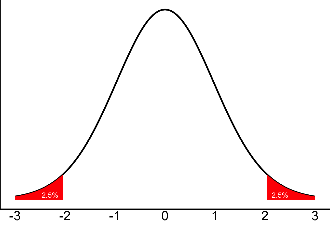
Step 3 is to determine the cutoff values for rejecting the null hypothesis. Use a t-table to look up the cutoff values for a two-tailed test when we’re asking is \(p<.05\) and have the \(df\) we discussed in the answer above.

What are the cutoff values?

Looking at a t-table should give you \(t_{crit}(30)=\pm2.04\).

We can add them onto the plot:

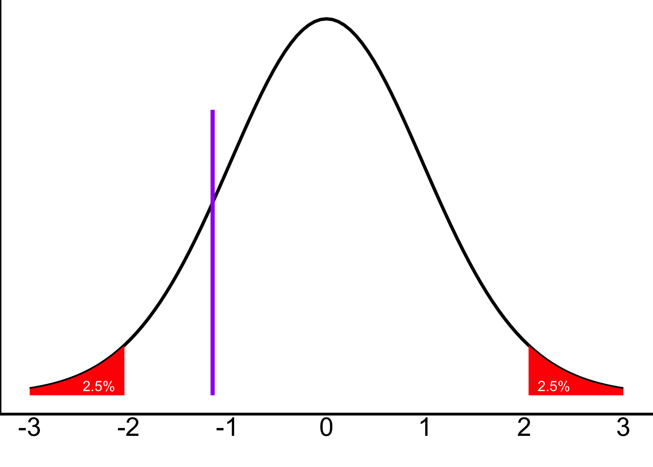
For step 4 (finding the t-score) and step 5 (comparing it to those cutoff values), we can just do this in Jamovi. (Remember, Jamovi doesn’t give you the critical t-value—it gives you a p-value, which answers the question for you.)

In Jamovi, click on Analyses, T-Tests, Independent Samples T-Test. Put shootingdrills into the Grouping Variable and expectedoutcome_4 into the Dependent Variable. Make sure Student’s t is selected.

Look over the results in Jamovi. Click below to see what your results should look like.

See the results and discuss what they mean

		Statistic	df	p
Independent Samples T-Test
expectedoutcome_4	Student's t	−1.15	30.0	0.259

The “Statistic” is the t-value. Here, it’s -1.15: negative, because our groups are ordered such that Jamovi did a smaller number minus a larger one. We also have the df, which we found above. And Jamovi gives us a p-value for the t-statistic. It’s not the \(t_{crit}\). It’s the actual p-value that your t corresponds to. So when \(t=-1.15\) for \(df=30\), Jamovi has looked up that it corresponds to a p-value under the null of 0.259. Your task is just to ask “is this p smaller than the p I was asking about, which here is 0.05?” And no, 0.259 is certainly not smaller than 0.05.

You can also click “Descriptives” under the T-Test menu in Jamovi, and it will give you the means of each group. This might be useful as you get into the last bit.

Practice writing up the results. Include the means of each group, whether the results are significant, and the results of the t-test. (You should follow what I have below in your answers for most of the questions today!)

Practice writing the results as we discussed in class, then click below to see my answer and a discussion.

There was no significant difference between groups. The shooting drills group (\(M = 74.2\)) showed no significant difference from the no-drills group (\(M = 53.43\)) in terms of how likely they were to vote this fall, \(t(30)=-1.15,p>.05\).

Those means are pretty far apart! But the groups are very different in size, and the standard deviation of the comparison distribution was quite large as we discussed above. So even a 20-ish point difference doesn’t mean much when the standard deviation is also close to 20 points.

We can add that _t_score into the plot from above:

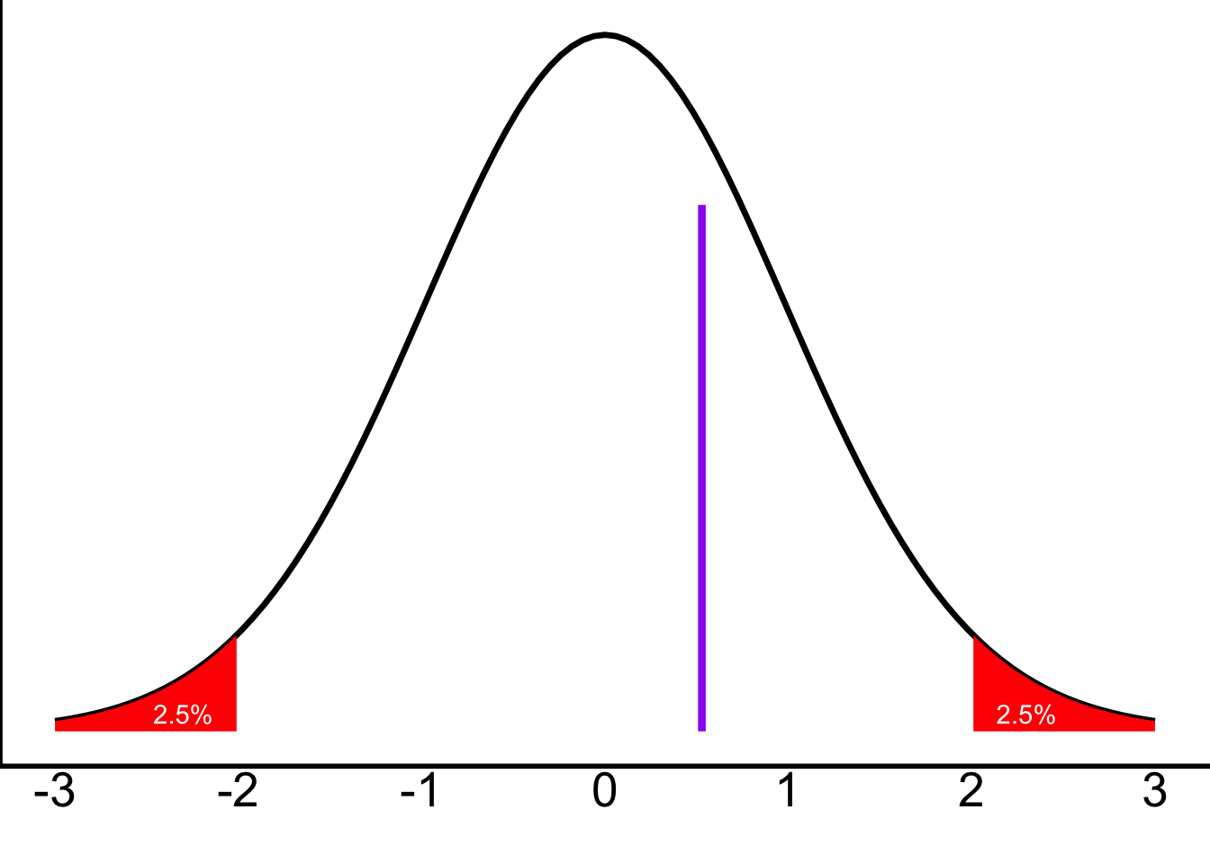
Visually, you should be able to see that this score falls within the null distribution; it isn’t extreme. Therefore, it makes sense that we have failed to reject the null.

Okay, now do these on your own.

With the friends data, use the cigarettes column (whether or not they’re a smoker) and the like.dance column (how much they like to dance). Is smoking a predictor of how much people like to dance? Use an independent-samples t-test. Write up your results. Use the steps of hypothesis-testing if that’s helpful. The important things to turn in for #1 are the results of the test and an answer to the question. Write up the results. (Not sure what I mean by “write up the results”? Do it like I did in the dropdown that says “Practice writing the results”.)
Are people with “natural” hair color more likely to vote than those with dyed hair? Use variables haircolor and expectedoutcome_4. (Hint: it will be close, but the answer is no. But if there were any results, it would probably be a fluke, right?) Write up the results, including the t-test, as #2.
Let’s look at the Schroeder & Epley data we discussed in class. Download it here or on Brightspace and load it into Jamovi. Re-run the test we discussed in class: does CONDITION predict Hire_Rating? (CONDITION is 1 and 0; 1 corresponds to Audio and 0 to Transcript.) Your resulting t-value will be negative. What does that mean? Answer this question, and include the t-test results, for #3. Then, try using the variable (lowercase) condition instead. It just has the CONDITION variable recoded to be a bit more meaningful. Why do you think the t is switched from negative to positive?

Repeat the test with the Intelect_Rating variable instead. Write up the results for #4.
Okay, now some quick practice for the exam. I’ll provide some numbers: the means for impression rating by groups are \(M=5.97\) for the audio group and \(M=4.07\) for the transcription group, the sample sizes are (as we discussed in class) \(n_1=21\) for the audio group and \(n_2=18\) for the transcription group, and the pooled variance is \(S_{\textrm{pooled}}^2=4.28\). Use those numbers and the formulae below this paragraph to calculate \(S_{\textrm{difference}}\) and t. Report that standard deviation of the distribution of the difference between the means (\(S_{\textrm{difference}}\)), and your t-value as answer #5. Also summarize the results of the t-test. You can use a t-table or to just also run this test (with the Impression_Rating variable) in Jamovi to confirm.

Remembering that the \(S_{\textrm{difference}}\) is the standard deviation of the distribution of the differences between means, the \(S_{\textrm{pooled}}^2\) is the pooled variance, and 1 and 2 refer to the samples:

\[S_{\textrm{difference}}=\mathit{SE}=\sqrt{S_{\textrm{pooled}}^2(\frac{1}{n_1}+\frac{1}{n_2})}~~\textrm{and}~~t=\frac{M_1-M_2}{S_{\mathrm{difference}}}\]

Finally, create a graph representing the results of at least one of these tests. Use Excel or Google Sheets, or play around with Jamovi to present the results in a way that makes sense. This is answer #6. Your graph should have labeled axes and include error bars (you could use SEM by group or the \(S_{difference}\) for error). While Jamovi can make these plots, you may want to practice creating them before next week.

Reuse

https://creativecommons.org/licenses/by/4.0/

Citation

BibTeX citation:

@online{dainer-best2024,
  author = {Dainer-Best, Justin},
  title = {\_T\_-Tests for Independent Means {(Lab} 6)},
  date = {2024-03-07},
  url = {https://faculty.bard.edu/jdainerbest/stats/labs//posts/06-t-tests},
  langid = {en}
}

For attribution, please cite this work as:

Dainer-Best, Justin. 2024. “_T_-Tests for Independent Means (Lab 6).” March 7, 2024. https://faculty.bard.edu/jdainerbest/stats/labs//posts/06-t-tests.