
| id | hrsd.pre | hrsd.post | hars.pre | hars.post | num.sessions |
|---|---|---|---|---|---|
| P003 | 16 | 3 | 15 | 4 | 9 |
| P004 | 16 | 7 | 33 | 13 | 12 |
| P006 | 13 | 8 | 13 | 6 | 11 |
| P007 | 11 | 3 | 17 | 4 | 14 |
| P009 | 17 | 7 | 9 | 11 | 12 |
| P012 | 9 | 0 | 13 | 1 | 8 |
| P013 | 14 | 3 | 19 | 6 | 10 |
| P014 | 10 | 3 | 12 | 6 | 9 |
| P019 | 10 | 5 | 10 | 3 | 7 |
| P023 | 8 | 1 | 7 | 2 | 10 |
| P040 | 21 | 8 | 41 | 9 | 13 |
| P048 | 14 | 6 | 17 | 8 | 11 |
| P068 | 11 | 6 | 14 | 12 | 9 |
| P072 | 15 | 6 | 13 | 4 | 8 |
| P074 | 12 | 8 | 10 | 11 | 10 |
| P075 | 18 | 11 | 23 | 18 | 8 |
| P100 | 7 | 2 | 14 | 1 | 4 |
| P111 | 18 | 11 | 15 | 8 | 13 |
| P115 | 18 | 8 | 19 | 8 | 9 |
| P117 | 12 | 9 | 18 | 7 | 8 |
| P127 | 9 | 4 | 13 | 5 | 12 |
| P139 | 14 | 9 | 12 | 9 | 14 |
| P160 | 13 | 6 | 11 | 3 | 13 |
| P163 | 16 | 10 | 16 | 5 | 14 |
| P169 | 13 | 9 | 15 | 3 | 12 |
| P202 | 10 | 4 | 11 | 7 | 12 |
| P203 | 18 | 5 | 20 | 10 | 10 |
| P206 | 11 | 2 | 16 | 4 | 9 |
| P219 | 21 | 5 | 27 | 9 | 10 |
| P220 | 14 | 10 | 13 | 9 | 12 |
| P223 | 21 | 3 | 12 | 2 | 9 |
| P244 | 12 | 3 | 8 | 3 | 10 |
Objectives
Today’s lab’s objectives are to:
- Learn about dependent-samples t-tests
- Learn how to conduct a dependent-samples t-test in Jamovi (and, a little bit, with the help of Jamovi)
- Visualize the results of such tests
There is no answer sheet for today’s lab. You’ll also complete a brief lab project today, which is due by next lab.
Dependent means t-tests
In a dependent means t-test, otherwise-known-as the t-test for dependent means, or a paired-samples t-test, we are comparing two means that are dependent on one another in some way. The scores are related to one another in a way that’s relatively easy to see—usually, e.g., because it’s the same person who’s doing something at two time-points.
As with the independent-samples t-test, the population’s mean and variance are unknown, and so must be estimated.
In the dependent-samples t-test, we can calculate difference scores with individuals because there is an obvious individual to subtract from—themself—and so we can easily do so. Rather than needing to use a distribution of the differences between means, we can use a single comparison distribution based on those difference scores.
Answer the following questions for yourself before clicking on them to see the answers.
NoteWhich is the comparison distribution for the t-test for dependent means?
The comparison distribution is a t distribution with a mean of 0 and SD of \(S_M\).
Why is the mean 0? Because the distribution is based on the difference scores for the paired scores. Under the null, there is no difference between time 1 and time 2 (or paired score 1 and paired score 2), so the mean of the comparison distribution is 0.
As with all of the tests we’ve discussed, the standard deviation of this comparison distribution is based on the standard error. Here, that’s \(S_M\), which is, like in the one-sample t-test, equal to \(S_M=\frac{S}{\sqrt{n}}\). S is of course the standard deviation, and n the sample size. Importantly, note that n is the sample size of the differences. So if there are 45 people who did a task twice, then \(n=45\). It’s not the total number of scores (45 and then 45 again).
NoteWhy is the df in a t-test for dependent means equal to n-1?
Because the paired samples mean that there’s more room for variation—only one of the sample scores needs to be constrained, while all of the others are “free to vary”. Again, the \(df=n-1\) refers to the sample size. If there are 45 participants who did a task twice, then \(df=45-1=44\).
NoteWhat is the formula for t in the t-test for dependent means?
\[t=\frac{M-\mu}{S_M}\]
It’s the same formula as for the one-sample t-test, based on the difference scores. So the \(M\) is the mean of the difference scores. The \(\mu\) is the mean of the difference scores under the null distribution, which is almost always going to be 0. And we discussed the \(S_M\) above.
Key ideas
So, the major takeaways here are:
The dependent-samples t-test is based on the difference scores, but because those difference scores are calculated within paired participants, the comparison distribution is based on the sampling distribution of those difference scores (rather than needing to compare the distribution of the difference between the means, as in an independent-samples t-test).
Therefore, this test has \(df=n-1\), like the one-sample t-test, and not \(df_\textrm{total}=n-2\), like in the t-test for independent means. Again, the \(n\) here is the number of participants (if a task is repeated twice) or the number of pairs (if linked in some other way).
The comparison distribution in the dependent-samples t-test is a t distribution with a mean of 0, \(df=n-1\), and a standard deviation based on the sampling distribution of difference scores. In the dependent-samples t-test, however, this distribution is just the sampling distribution created after subtracting each pair. The standard deviation of this comparison distribution is based on the difference score distribution’s own \(SD\) and \(n\) (\(S_M=\frac{S}{\sqrt{n}}\)). No pooling is necessary because we treat this as a single distribution.
The cutoff for the sample is based on those degrees of freedom, e.g., \(\pm2.78\) (i.e., -2.78, 2.78) for \(df=4\).
The equation for t has not substantially changed: \(t=\frac{M-\mu}{S_M}\)—and in fact, \(\mu\) in the dependent-samples t-test is pretty much always actually equal to 0, because we are pretty much always testing whether there is a difference between our two groups (if there’s a significant difference from 0). So you can even simplify it to be \(t=\frac{M}{S_M}\) (if you recall that subtracting 0 is, well, no change). The M is the mean of the difference scores.
I’ve suggested that it’s quite easy to identify whether a test should require a t-test for dependent means, or not—because the test obviously includes paired samples. Let’s give it a try. For each of the following, select which kind of test is best. (These include all of the tests we’ve discussed in class—both z and t.)
NoteA researcher wants to test whether the average score on a certain exam taken by college students is different from the average score on the same exam when taken by the general population. The population standard deviation of is known. What type of test should the researcher use?
This is a z-test for a sample. We know something about the ‘average’ person (i.e., the population mean), and want to compare a sample to them. We also know the population standard deviation, so can use a z-test.
NoteA researcher wants to test whether a new drug is effective in reducing anxiety levels. The researcher randomly assigns participants to either receive the new drug or a placebo. What type of test should the researcher use to compare the anxiety levels of the two groups?
Here, you should use a t-test for independent means. We have people who are being measured in one group, and some who are being measured in another. We don’t know anything about the population mean or SD. A t-test is therefore appropriate. But they’re not linked, so it’s not dependent-samples.
NoteA researcher wants to test whether a new teaching method is effective in improving student performance. The researcher randomly assigns students to either receive the new teaching method or the traditional teaching method. What type of test should the researcher use to compare the performance of the two groups?
This is also t-test for independent means. Again, there are two unmatched groups. Some students receive the new method, while others receive the traditional one. We know nothing about the population.
NoteA researcher wants to test whether there is a relationship on a test of class-specific knowledge. The researcher gives an exam of important class topics before beginning the semester, and then gives the same exam again at the final. What type of test should the researcher use to measure whether students know more after the class is over?
This is a t-test for dependent means. We know nothing about the population, and have one samples being measured twice. Because there is one, matched group, we can use the test for dependent means and be focused on the difference scores.
NoteYou want to compare whether one particular individual has a different level of oxytocin compared to the general population.
This is probably a z-test for a single score. I haven’t told you if we know the population’s mean and SD, but you know we’re comparing them to the general population. You can’t use a t-test for a case like this. If you don’t know the general population’s mean and variance, you couldn’t make any comparison at all.
NoteA researcher is interested in whether monozygotic (‘identical’) twins have the same level of neuroticism as one another at the age of four.
This is probably a t-test for dependent means. The samples are paired (each twin with its sibling) and therefore the test is paired. Although it’s not the same person, the nature of the question has a pairing. You might see something similar in questions about monogamous romantic partners, too.
Nice work! Feel free to explore why which test is being used with your classmate or with the instructor. Then get into doing some tests!
First test
Today we’ll be using data from a study from 2019, Fisher et al. (2019) (link to read article). The data from Fisher and colleagues was a test of a type of therapy they had developed; read more at the link. For all participants, the researchers collected Hamilton Rating Scale for Depression (HRSD) and Hamilton Anxiety Rating Scale (HARS) before and after treatment. Let’s take a look (you can scroll down):
Download the data here. Open it in Jamovi.
You’re going to use the Compute function under Data. Create two columns of difference scores (for post-treatment MINUS pre-treatment scores), for both the HARS and HRSD. Be sure to pay attention to the names of the columns (hars.pre and hars.post; hrsd.pre and hrsd.post). You’ll use a - (minus) to subtract, as should make sense! (Questions about this compute function? Read more here).
Subtracting the pre (before) scores from the post (after scores) gives us a negative score when scores have gone down (from pre to post) and a positive score when scores have gone up.
Your dataset should now have two columns that look like this (as well as the previous columns):
| id | hrsd.diff | hars.diff |
|---|---|---|
| P003 | -13 | -11 |
| P004 | -9 | -20 |
| P006 | -5 | -7 |
| P007 | -8 | -13 |
| P009 | -10 | 2 |
| P012 | -9 | -12 |
| P013 | -11 | -13 |
| P014 | -7 | -6 |
| P019 | -5 | -7 |
| P023 | -7 | -5 |
| P040 | -13 | -32 |
| P048 | -8 | -9 |
| P068 | -5 | -2 |
| P072 | -9 | -9 |
| P074 | -4 | 1 |
| P075 | -7 | -5 |
| P100 | -5 | -13 |
| P111 | -7 | -7 |
| P115 | -10 | -11 |
| P117 | -3 | -11 |
| P127 | -5 | -8 |
| P139 | -5 | -3 |
| P160 | -7 | -8 |
| P163 | -6 | -11 |
| P169 | -4 | -12 |
| P202 | -6 | -4 |
| P203 | -13 | -10 |
| P206 | -9 | -12 |
| P219 | -16 | -18 |
| P220 | -4 | -4 |
| P223 | -18 | -10 |
| P244 | -9 | -5 |
Once it does, let’s continue! (And it’s fine if all of your scores are the opposite direction, e.g., 9 instead of -9.) The questions we could ask with a t-test are these: Did participants improve on depression? What about on anxiety?
We’ll start by doing this by hand (i.e., using the formulas you’ve learned and which were discussed above), and then get into doing it with the t-test function in Jamovi.
Step 1: Restate question as a research and null hypothesis
NoteWhat are the null and research hypotheses?
Null: There is no difference between the means for participants before treatment and after treatment, \(\mu_{difference}=0\)
You could also think about this as the pre and post being equivalent, \(\mu_{pre}=\mu_{post}\)
Research: There is a significant difference between the means for participants before treatment and after treatment, \(\mu_{difference}\neq0\)
You could also think about this as the pre and post being different, \(\mu_{pre}\neq\mu_{post}\)
Step 2: Determine the characteristics of the comparison distribution
To get more information from the difference scores between pre- and post- HRSD scores, we’ll use those hrsd.diff scores you calculated. Find the mean in Jamovi (Analyses: Exploration: Descriptives). Find the standard deviation. Find the n, and write down the df.
Lastly, we need the \(S_M\), the standard deviation for the comparison t distribution. Recall that \(S_M=\frac{S}{\sqrt{n}}\)… we have s and n, so you can calculate that!
NoteConfirm your numbers
The mean is -8.03125 and SD is 3.5964532. Rounding, Jamovi gives \(M_{HRSD_{pre-post}}=-8.03\) and \(SD_{HRSD_{pre-post}}=3.60\). \(n=32\) and therefore \(df=n-1=31\).
\(S_M=\frac{S}{\sqrt{n}}=0.64\)
Okay, so what does the t distribution look like for this comparison? Like this:
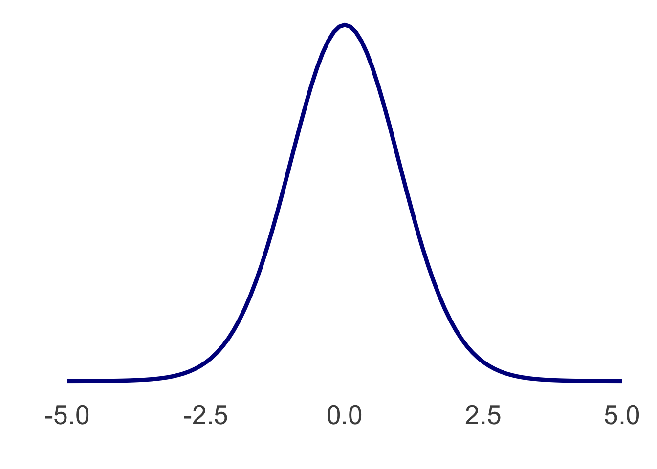
It’s sort of normal—although not quite—and it has 31 degrees of freedom, a mean of 0, and a standard deviation of the \(S_M\) you just calculated.
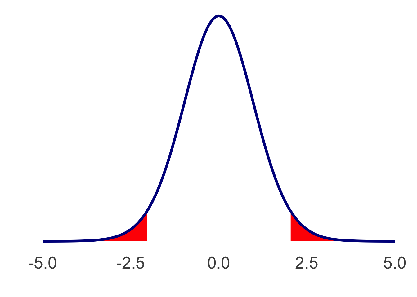
Step 3: Determine the sample cutoff score
This step hasn’t changed from last time we discussed it; you could use your t-table with the degrees of freedom you found. I’ll tell you that the cutoff score, based on \(df=31\) is \(\pm2.04\).
This gives us a plot like the following:
Step 4: Determine the sample’s [t] score
Well, we’ve got all the pieces that go into the t equation:
\[t=\frac{M-\mu}{S_M}\]
Write out the t equation with each of those variables replaced with your numbers. Then solve it and find t.
NoteCheck your value for t
\(t=\frac{M-\mu}{S_M}=\frac{-8.03-0}{0.64}=(-8.03-0)/0.64=-12.55\). That said, without any rounding, it might be more like \((-8.03125-0)/0.6357691=-12.632\)
You may have gotten anywhere in the middle. Jamovi will give you an answer that is only rounded at the end.
Step 5: Determine whether to reject the null
Your eye can probably tell you whether we can reject the null. But, formally: is it larger than 2.04 or smaller than -2.04?
NoteDo we reject the null?
Yes, -12.63 is much more extreme (further from 0) than the cutoff value of -2.04. (Or, if you did it in a positive direction, it’s much more extreme than the cutoff value of +2.04.)
Do it with a function in Jamovi
So, the great thing about modern software is that we very rarely need to calculate things like this step-by-step. Instead, you can use the functions in Jamovi. You might recall that I said that the t-test for dependent means is essentially the t-test for a single sample whose population mean is 0, if you find the difference scores. Well, we calculated the difference scores, in the column hrsd.diff. So you can try running this as a t-test for a single sample.
In Jamovi, run a one-sample t-test on the HRSD difference scores. You don’t need to change anything, since the Test value (under Hypothesis) by default is 0. Did you get something very close to the t-score you calculated? You should have.
Now, do it with the paired-samples test, which doesn’t require calculating difference scores (Analyses -> T-Tests -> Paired Samples T-Test). Put hrsd.pre and hrsd.post into the “paired variables” box. Do you get the same value? You should!
Most of the time, we don’t actually calculate the difference scores—we run the paired samples t-test to think about the means of each pair, separately.
Do note that Jamovi expects there to be two columns here, so it knows how the data are paired. (It assumes that each row is “paired” which is usually right.) If for some reason you had data in another format, like what you see below, you would need to restructure it:
| id | time | hrsd |
|---|---|---|
| P003 | pre | 16 |
| P003 | post | 3 |
| P004 | pre | 16 |
| P004 | post | 7 |
| P006 | pre | 13 |
| P006 | post | 8 |
| P007 | pre | 11 |
| P007 | post | 3 |
| P009 | pre | 17 |
| P009 | post | 7 |
| P012 | pre | 9 |
| P012 | post | 0 |
| P013 | pre | 14 |
| P013 | post | 3 |
| P014 | pre | 10 |
| P014 | post | 3 |
| P019 | pre | 10 |
| P019 | post | 5 |
| P023 | pre | 8 |
| P023 | post | 1 |
| P040 | pre | 21 |
| P040 | post | 8 |
| P048 | pre | 14 |
| P048 | post | 6 |
| P068 | pre | 11 |
| P068 | post | 6 |
| P072 | pre | 15 |
| P072 | post | 6 |
| P074 | pre | 12 |
| P074 | post | 8 |
| P075 | pre | 18 |
| P075 | post | 11 |
| P100 | pre | 7 |
| P100 | post | 2 |
| P111 | pre | 18 |
| P111 | post | 11 |
| P115 | pre | 18 |
| P115 | post | 8 |
| P117 | pre | 12 |
| P117 | post | 9 |
| P127 | pre | 9 |
| P127 | post | 4 |
| P139 | pre | 14 |
| P139 | post | 9 |
| P160 | pre | 13 |
| P160 | post | 6 |
| P163 | pre | 16 |
| P163 | post | 10 |
| P169 | pre | 13 |
| P169 | post | 9 |
| P202 | pre | 10 |
| P202 | post | 4 |
| P203 | pre | 18 |
| P203 | post | 5 |
| P206 | pre | 11 |
| P206 | post | 2 |
| P219 | pre | 21 |
| P219 | post | 5 |
| P220 | pre | 14 |
| P220 | post | 10 |
| P223 | pre | 21 |
| P223 | post | 3 |
| P244 | pre | 12 |
| P244 | post | 3 |
(You can’t do this easily in Jamovi. Or, you can, but you need to install a Module called jTransform to do it.)
An additional thing to again notice about the test you ran in Jamovi: the degrees of freedom are based on the participants, not the number of scores. If this was an independent-samples test, we’d see \(df=62\) but because they’re matched, we only have one person’s difference scores which must be constrained.
Okay, two more things:
First, let’s write up a report of our results.
Practice writing up the results of your t-test on the HRSD scores. Include the means pre- and post-, and the actual test results in the format of t(df)=t-value, p < .05 (or p > .05—in this case, it is indeed \(p<.05\)). Replace df and t-value with the values from the test, and pick one of the options for p. Then, very briefly, explain your results. Is there a directional effect? Was this statistically-significant? What does it mean?
NoteSee how I wrote this up (click to expand)
Depression scores dropped from baseline (\(M=13.8\)) to post-treatment (\(M=5.78\)) on the HRSD, \(t(31)=-12.6,p<.05\).
You could also write “The results were statistically-significant”, but the key is having the test, showing that \(p<.05\), and understanding that it indicates a reduction in depression scores. Keeping it brief is great!
Note what we don’t need to include: these reports do not include the \(t_{crit}\) (the critical t-value is used to compare our t-score, and therefore to decide “is \(p<.05\)?”, not to report). We also don’t usually include the actual p-value, as I’ve said, just whether it is less than .05. We just include the \(df\) and t-score, and the conclusions of the test.
Now, in Jamovi, and under the paired samples t-test menu, click “Descriptives plots.” Then look at the following plot, which you would need to restructure your data in Jamovi to create. Try plotting a bar graph of the HRSD data in Jamovi and you’ll see why—even after you set the variables hrsd.pre and hrsd.post to continuous, the bar plot will plot them separately.
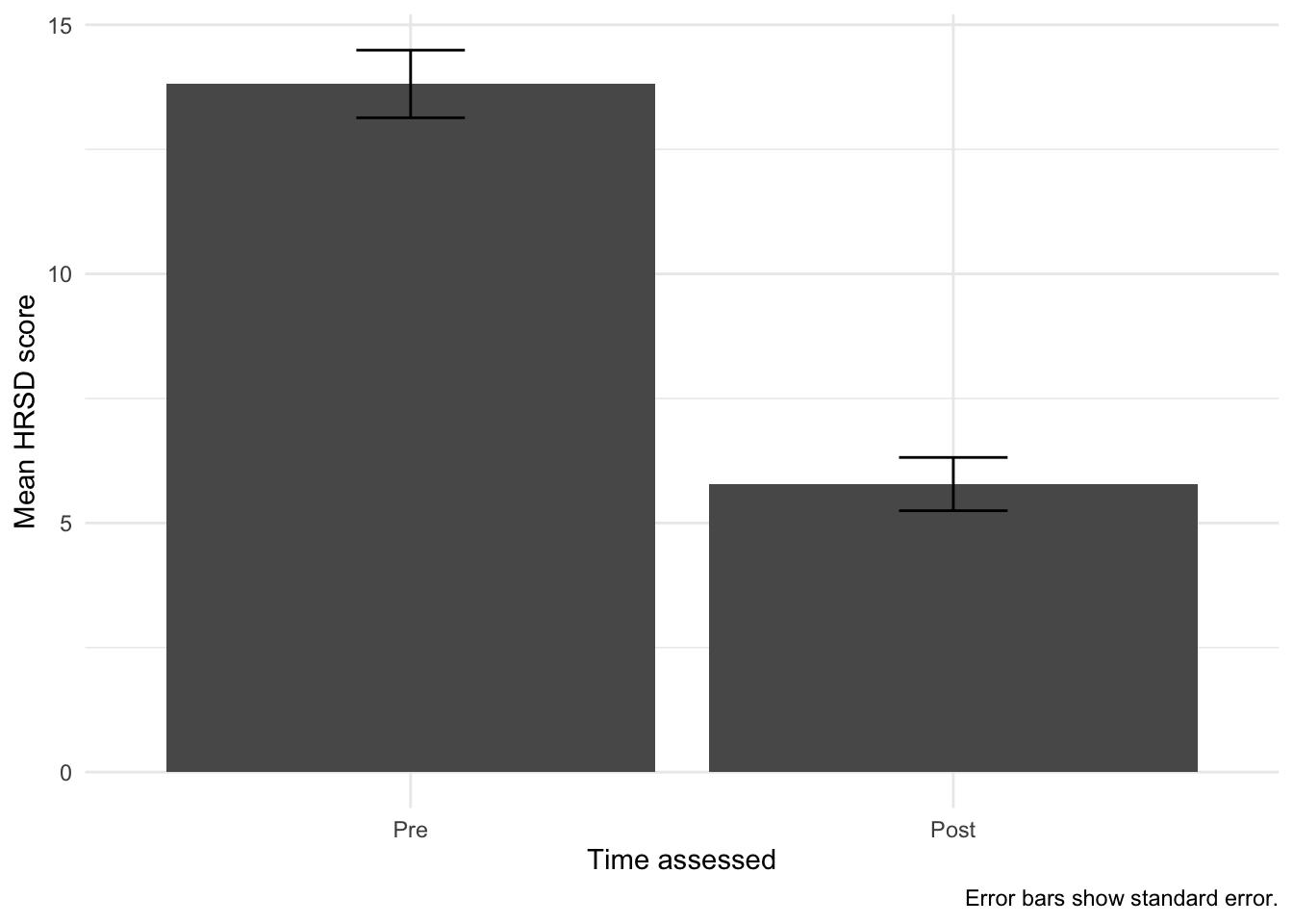
Think about the differences between the plots. What do they tell you? Do you have a preference?
The plot I include here shows a bar graph, which shows the means and is similar to the ones you can get from the Descriptives menu in Jamovi (or make in Excel or Google Sheets). The Jamovi plot that it gives with the t-test is just points, but shows both the means and the medians. Both plots have error bars; the Jamovi plot is labeled and says they’re 95% confidence intervals, whereas the plot above shows error bars with standard error. Both show the means and possible variation around them. The plot on this page has labeled axes and somewhat clearer descriptions (but you could edit the Jamovi one if you needed to). You could also get the Descriptives in Jamovi and take them to Excel or Sheets to make a bar graph.
You could also either learn to use the jTransform “Wide to Long” function (see below—it’s finicky but doable) or copy the data into Excel. In this particular case, you can just copy the data above (I gave it to you in this format, with columns of id, timepoint, and HRSD) into a new Jamovi window, and then plot it using a bar plot.
NoteLearn to use “Wide to Long” in the jTransform module in Jamovi (click to expand)
Click on Modules (at the right of the Jamovi window). Then click Jamovi library. Type in jTransform and install it.
With your fisher data open, click on the Data tab. Make the HRSD and HARS variables all into Continuous data types. Make ID into an ID data type.
Now, click on the new module under Analyses (Data) and select “Wide to Long”. We want the Separated tab under Mode, which should be where it starts—our variable names are separated by a period (e.g., hrsd.pre has hrsd separated from pre by a period).
- Put
idinto “Variables that identify the same unit”. - Under “Variables to be transformed”, put
hrsd.pre,hrsd.post,hars.pre, andhars.post. - Under “Variables not to be transformed”, put
num.sessions - Leave the
hars.diffandhrsd.diffvariables alone. - Below, under Prefix, type
time– this is . Under Separator, change it from_to.– (there’s a period separating the variable names). Leave Exclude Level blank. - If you’ve done everything right, it will give you a preview of your new data. Click Create. A new dataset will open in Jamovi.
Rename the new variables: time1 should be called scale and time2 should be named time. You should move the pre level of time to be FIRST as well. Now, you can plot these data in a bar plot: Go to Analyses: Exploration: Descriptives. Put measure into the Variables and put both scale and time into the Split By—time should be above scale. Turn on the bar plot under Plots. You should get a plot that looks like this:
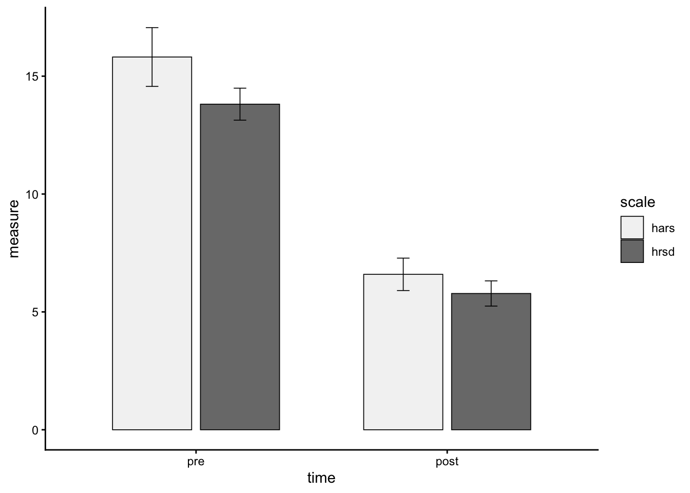
You can reverse the order in the Split By part of the Jamovi analysis in order to see the bars grouped by measure. You could also filter (in Data) to only hars (measure == "hars"), then to only hrsd (measure == "hrsd"), to make separate plots.
There is additional information on this in a Jamovi doc on reshaping datasets.
Try again with HARS
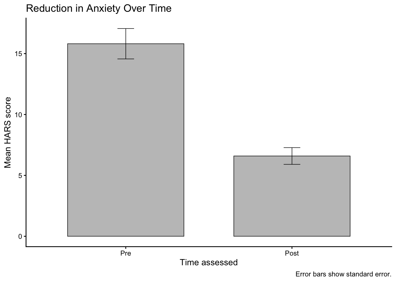
We tested the Fisher dataset’s depression scale, HRSD, but not the anxiety scale, HARS. Did anxiety significantly decrease during treatment? Do a dependent-samples t-test to find out and report the results. Do it however you like, by hand or with Jamovi, but use the steps of hypothesis-testing in your mind. Do think through what the comparison distribution is, practice getting the results of the test, and writing a concluding sentence or two.
Then click through and see my summary.
NoteSummary of HARS test
Step 1: Define hypotheses
Null: There is no difference between anxiety scores before and after treatment, \(\mu_{pre}=\mu_{post}\) and \(\mu_{difference}=0\)
Research hypothesis: There is a difference between anxiety scores before and after treatment, \(\mu_{pre}\neq\mu_{post}\) and \(\mu_{difference}\neq0\)
Step 2: Determine the characteristics of the comparison distribution
Because this is a dependent-samples t-test, the comparison distribution is the t distribution. The degrees of freedom will be equal to \(n-1\), the mean will be 0, and the \(S_M\) will be the standard deviation of the difference distribution.
Therefore, \(df=31\), \(\mu_M=0\), and \(S_M\) is the SEM.
Here, \(S_M=1.12\).
Steps 3, 4, and 5
We’ll integrate the last three steps into the running of the t-test:
| statistic | df | p | |||
|---|---|---|---|---|---|
| hars.pre | hars.post | Student's t | 8.21 | 31.0 | <.001 |
Even though this reports p as “< .001,” you should report the answer to our question: yes, \(p<.05\).
Yes, there is a significant difference—a reduction in anxiety scores, such that participants had a mean score of \(M=15.80\) before treatment and \(M=6.59\) after treatment; there is a statistically significant result for a dependent means t-test, \(t(31)=8.21, p < .05\).
Reuse
Citation
BibTeX citation:
@online{dainer-best2025,
  author = {Dainer-Best, Justin},
  title = {\_T\_-Tests for Dependent Means {(Lab} 7)},
  date = {2025-10-16},
  url = {https://faculty.bard.edu/jdainerbest/stats/labs/posts/07-dependent-t-tests/},
  langid = {en}
}
For attribution, please cite this work as:
Dainer-Best, Justin. 2025. “_T_-Tests for Dependent Means (Lab
7).” October 16, 2025. https://faculty.bard.edu/jdainerbest/stats/labs/posts/07-dependent-t-tests/.