
| Condition | Time_of_Day | BDI_II | STAI_T | pre_film_VAS_Sad | pre_film_VAS_Hopeless | pre_film_VAS_Depressed | pre_film_VAS_Fear | pre_film_VAS_Horror | pre_film_VAS_Anxious | post_film_VAS_Sad | post_film_VAS_Hopeless | post_film_VAS_Depressed | post_film_VAS_Fear | post_film_VAS_Horror | post_film_VAS_Anxious | Attention_Paid_to_Film | Post_film_Distress | Day_Zero_Number_of_Intrusions | Days_One_to_Seven_Number_of_Intrusions | Visual_Recognition_Memory_Test | Verbal_Recognition_Memory_Test | Number_of_Provocation_Task_Intrusions | Diary_Compliance | IES_R_Intrusion_subscale | Tetris_Total_Score | Self_Rated_Tetris_Performance | Tetris_Demand_Rating |
|---|---|---|---|---|---|---|---|---|---|---|---|---|---|---|---|---|---|---|---|---|---|---|---|---|---|---|---|
| 1 | 2 | 1 | 33 | 0.0 | 0.0 | 0.0 | 0.4 | 0.3 | 0.8 | 1.0 | 0.3 | 0.0 | 0.3 | 0.6 | 1.2 | 9 | 8 | 2 | 4 | 15 | 18 | 5 | 9 | 0.62 | NA | NA | 0 |
| 1 | 2 | 3 | 27 | 1.9 | 0.7 | 0.5 | 0.8 | 0.2 | 0.2 | 1.1 | 0.4 | 0.4 | 2.0 | 5.8 | 5.5 | 10 | 2 | 2 | 3 | 17 | 19 | 4 | 9 | 0.62 | NA | NA | 0 |
| 1 | 1 | 10 | 42 | 2.2 | 1.2 | 0.9 | 0.2 | 0.1 | 0.4 | 6.7 | 2.0 | 1.0 | 0.7 | 3.1 | 0.4 | 10 | 6 | 5 | 6 | 12 | 21 | 0 | 10 | 0.50 | NA | NA | 0 |
| 1 | 1 | 1 | 41 | 1.2 | 1.0 | 0.6 | 5.1 | 0.4 | 0.5 | 5.1 | 0.6 | 1.8 | 5.3 | 3.2 | 3.6 | 9 | 8 | 0 | 2 | 16 | 19 | 0 | 8 | 0.50 | NA | NA | 3 |
| 1 | 2 | 1 | 27 | 0.2 | 0.1 | 0.0 | 2.9 | 0.0 | 0.7 | 4.0 | 0.0 | 0.0 | 8.4 | 7.0 | 8.4 | 10 | 7 | 5 | 3 | 14 | 22 | 10 | 8 | 1.00 | NA | NA | -7 |
| 1 | 1 | 1 | 25 | 1.6 | 0.7 | 0.0 | 0.6 | 0.6 | 0.6 | 4.0 | 0.4 | 0.9 | 4.0 | 4.9 | 6.6 | 9 | 8 | 4 | 4 | 13 | 15 | 0 | 9 | 0.88 | NA | NA | -2 |
| 1 | 2 | 0 | 25 | 0.0 | 0.0 | 0.0 | 0.0 | 0.0 | 0.1 | 0.0 | 0.0 | 4.4 | 2.0 | 1.7 | 1.8 | 10 | 8 | 0 | 0 | 15 | 19 | 1 | 10 | 0.00 | NA | NA | 0 |
| 1 | 1 | 4 | 46 | 0.5 | 2.1 | 0.5 | 0.5 | 0.3 | 0.1 | 7.6 | 3.9 | 6.9 | 1.4 | 3.9 | 0.6 | 10 | 9 | 4 | 4 | 16 | 16 | 7 | 8 | 0.38 | NA | NA | 2 |
| 1 | 2 | 0 | 21 | 0.3 | 0.1 | 0.1 | 0.0 | 0.0 | 0.0 | 4.8 | 0.4 | 3.9 | 0.0 | 2.5 | 0.0 | 10 | 7 | 3 | 2 | 13 | 22 | 5 | 9 | 0.38 | NA | NA | 0 |
| 1 | 1 | 11 | 58 | 0.7 | 1.0 | 0.7 | 0.0 | 0.0 | 0.6 | 2.5 | 1.1 | 1.2 | 1.8 | 3.1 | 7.0 | 9 | 7 | 5 | 11 | 20 | 23 | 3 | 8 | 1.75 | NA | NA | 5 |
| 1 | 2 | 0 | 25 | 0.5 | 0.9 | 0.6 | 0.0 | 0.0 | 1.6 | 1.9 | 3.0 | 0.7 | 7.7 | 6.5 | 8.1 | 10 | 7 | 5 | 16 | 13 | 18 | 3 | 9 | 0.75 | NA | NA | -1 |
| 1 | 2 | 8 | 41 | 2.6 | 0.6 | 0.9 | 0.0 | 0.0 | 0.0 | 6.9 | 1.2 | 6.6 | 1.1 | 5.0 | 0.3 | 9 | 8 | 5 | 12 | 15 | 21 | 2 | 8 | 1.13 | NA | NA | -3 |
| 1 | 2 | 1 | 30 | 0.3 | 1.2 | 2.0 | 0.0 | 0.0 | 1.0 | 2.5 | 0.4 | 0.8 | 0.4 | 6.8 | 1.0 | 10 | 3 | 1 | 2 | 15 | 20 | 7 | 9 | 0.38 | NA | NA | -4 |
| 1 | 1 | 0 | 34 | 0.0 | 0.8 | 0.0 | 1.1 | 0.7 | 1.0 | 0.0 | 0.0 | 0.0 | 0.6 | 0.5 | 0.5 | 10 | 5 | 5 | 7 | 18 | 20 | 4 | 9 | 1.50 | NA | NA | -3 |
| 1 | 2 | 4 | 27 | 0.0 | 0.0 | 0.0 | 0.0 | 0.0 | 0.0 | 1.0 | 0.0 | 0.0 | 0.0 | 1.3 | 2.9 | 10 | 4 | 4 | 7 | 17 | 22 | 5 | 7 | 1.25 | NA | NA | -3 |
| 1 | 2 | 15 | 48 | 1.1 | 0.0 | 1.1 | 1.2 | 0.4 | 0.8 | 2.2 | 1.9 | 3.5 | 3.0 | 4.0 | 1.5 | 10 | 6 | 3 | 6 | 13 | 18 | 2 | 8 | 2.25 | NA | NA | -5 |
| 1 | 1 | 0 | 29 | 1.2 | 0.0 | 0.0 | 0.0 | 0.0 | 1.5 | 1.0 | 0.4 | 0.7 | 0.0 | 2.6 | 1.0 | 10 | 6 | 1 | 2 | 15 | 20 | 0 | 9 | 0.25 | NA | NA | -3 |
| 1 | 2 | 0 | 22 | 0.0 | 0.0 | 0.0 | 0.4 | 0.4 | 0.3 | 1.0 | 0.0 | 0.0 | 3.8 | 5.7 | 6.8 | 9 | 7 | 10 | 1 | 13 | 23 | 3 | 7 | 0.50 | NA | NA | -3 |
| 2 | 2 | 8 | 46 | 0.0 | 0.0 | 0.0 | 0.0 | 0.0 | 0.4 | 7.4 | 0.0 | 3.4 | 0.5 | 2.2 | 0.3 | 10 | 6 | 3 | 1 | 16 | 21 | 0 | 9 | 1.50 | 16413 | 6.0 | -2 |
| 2 | 1 | 2 | 29 | 0.5 | 0.0 | 0.0 | 2.3 | 0.0 | 0.9 | 1.0 | 0.0 | 0.0 | 0.5 | 1.7 | 1.3 | 8 | 6 | 2 | 2 | 16 | 19 | 0 | 8 | 0.75 | 3231 | 5.4 | -1 |
| 2 | 1 | 0 | 36 | 0.4 | 0.9 | 0.5 | 2.0 | 0.7 | 3.0 | 4.7 | 0.6 | 1.3 | 3.1 | 5.0 | 4.8 | 9 | 6 | 9 | 3 | 19 | 15 | 0 | 8 | 1.25 | 12505 | 4.7 | -5 |
| 2 | 2 | 6 | 42 | 1.8 | 1.3 | 0.4 | 1.2 | 0.3 | 2.7 | 5.7 | 0.5 | 2.0 | 3.9 | 4.2 | 4.1 | 8 | 6 | 2 | 0 | 13 | 18 | 0 | 9 | 0.13 | 20567 | 3.1 | -6 |
| 2 | 2 | 0 | 25 | 0.3 | 2.2 | 0.3 | 1.0 | 0.5 | 5.6 | 4.7 | 2.2 | 3.2 | 3.3 | 4.9 | 4.3 | 10 | 7 | 2 | 2 | 18 | 20 | 3 | 10 | 0.75 | 4816 | 4.8 | -1 |
| 2 | 2 | 2 | 38 | 0.0 | 0.0 | 0.0 | 0.0 | 0.0 | 0.9 | 0.0 | 0.0 | 0.0 | 0.0 | 5.0 | 1.4 | 10 | 6 | 2 | 3 | 16 | 16 | 2 | 10 | 0.25 | 24233 | 1.8 | 8 |
| 2 | 2 | 5 | 31 | 0.2 | 0.2 | 0.0 | 0.2 | 0.0 | 1.4 | 5.7 | 0.5 | 1.3 | 5.2 | 1.6 | 6.0 | 9 | 8 | 3 | 2 | 16 | 20 | 4 | 8 | 0.63 | 22672 | 1.8 | -6 |
| 2 | 1 | 4 | 39 | 1.5 | 0.0 | 1.1 | 0.0 | 0.0 | 0.0 | 7.3 | 5.1 | 5.2 | 0.0 | 0.0 | 0.0 | 10 | 8 | 5 | 1 | 13 | 17 | 6 | 9 | 0.88 | 44650 | 1.8 | -2 |
| 2 | 1 | 1 | 34 | 0.5 | 0.2 | 0.0 | 0.3 | 0.2 | 3.8 | 1.9 | 0.7 | 0.2 | 2.9 | 6.1 | 6.4 | 10 | 8 | 2 | 7 | 18 | 22 | 1 | 9 | 0.38 | 90077 | 3.6 | -4 |
| 2 | 2 | 4 | 26 | 1.2 | 0.7 | 0.7 | 0.2 | 0.3 | 0.5 | 5.5 | 1.2 | 1.0 | 2.3 | 5.0 | 6.2 | 8 | 5 | 1 | 0 | 17 | 19 | 3 | 8 | 0.38 | 21648 | 2.7 | 0 |
| 2 | 2 | 0 | 30 | 0.7 | 0.5 | 0.3 | 0.2 | 0.1 | 0.1 | 1.9 | 0.6 | 0.3 | 0.2 | 0.2 | 0.2 | 9 | 4 | 1 | 3 | 13 | 19 | 1 | 9 | 0.38 | 26590 | 2.0 | 0 |
| 2 | 2 | 3 | 36 | 0.5 | 1.0 | 0.4 | 0.0 | 0.0 | 0.0 | 4.6 | 3.3 | 3.0 | 2.6 | 2.9 | 1.6 | 8 | 5 | 8 | 2 | 18 | 17 | 0 | 5 | 0.50 | 29027 | 3.0 | -4 |
| 2 | 1 | 2 | 27 | 0.5 | 0.4 | 0.5 | 0.1 | 0.2 | 1.6 | 1.6 | 0.7 | 1.2 | 4.1 | 7.6 | 4.5 | 10 | 10 | 2 | 2 | 12 | 18 | 0 | 6 | 0.50 | 53526 | 0.6 | 5 |
| 2 | 2 | 1 | 42 | 0.9 | 0.2 | 0.0 | 0.4 | 0.3 | 0.7 | 2.6 | 0.6 | 0.7 | 3.3 | 8.5 | 4.7 | 9 | 3 | 4 | 1 | 16 | 16 | 0 | 9 | 0.38 | 107782 | 1.2 | 0 |
| 2 | 1 | 0 | 37 | 0.0 | 0.0 | 0.0 | 0.6 | 0.0 | 3.2 | 2.0 | 2.1 | 0.0 | 0.0 | 9.5 | 9.0 | 10 | 6 | 1 | 0 | 16 | 18 | 0 | 9 | 0.50 | 34285 | 1.6 | -3 |
| 2 | 2 | 5 | 51 | 1.3 | 6.8 | 2.3 | 0.0 | 0.0 | 0.0 | 6.4 | 2.1 | 3.7 | 0.0 | 1.8 | 0.0 | 10 | 8 | 3 | 1 | 14 | 20 | 0 | 3 | 1.00 | 1425 | 2.2 | 0 |
| 2 | 1 | 0 | 24 | 0.0 | 0.0 | 0.0 | 0.7 | 0.5 | 0.4 | 2.8 | 0.0 | 1.4 | 0.9 | 3.0 | 2.1 | 10 | 8 | 2 | 0 | 13 | 18 | 0 | 10 | 0.00 | 32853 | 1.2 | -7 |
| 2 | 1 | 5 | 31 | 0.1 | 0.7 | 0.5 | 1.6 | 1.4 | 1.1 | 3.0 | 0.0 | 0.3 | 2.4 | 2.3 | 3.2 | 9 | 6 | 4 | 4 | 18 | 17 | 0 | 8 | 0.88 | 26885 | 5.7 | -4 |
| 3 | 1 | 5 | 27 | 1.6 | 0.6 | 0.0 | 2.5 | 0.1 | 1.3 | 4.6 | 7.7 | 1.5 | 1.9 | 4.3 | 2.0 | 10 | 9 | 4 | 2 | 15 | 25 | 5 | 9 | 0.50 | 27116 | 2.4 | -6 |
| 3 | 1 | 1 | 28 | 1.0 | 0.6 | 0.4 | 0.0 | 0.0 | 0.0 | 2.3 | 0.8 | 1.1 | 1.2 | 2.3 | 1.8 | 10 | 7 | 0 | 2 | 10 | 15 | 0 | 10 | 0.25 | 14360 | 2.1 | 2 |
| 3 | 2 | 0 | 21 | 0.0 | 0.1 | 0.0 | 0.3 | 0.7 | 1.1 | 1.5 | 0.0 | 1.0 | 1.1 | 2.5 | 1.2 | 10 | 8 | 6 | 2 | 15 | 17 | 0 | 10 | 0.87 | 37782 | 1.6 | 0 |
| 3 | 2 | 6 | 27 | 0.0 | 3.1 | 0.0 | 1.3 | 0.4 | 4.5 | 3.9 | 6.2 | 2.6 | 1.3 | 0.9 | 2.7 | 10 | 4 | 3 | 3 | 13 | 24 | 0 | 10 | 0.50 | 1035 | 5.5 | 0 |
| 3 | 2 | 18 | 53 | 0.0 | 0.0 | 0.0 | 0.0 | 0.0 | 0.0 | 0.0 | 0.0 | 0.0 | 2.9 | 5.8 | 2.3 | 10 | 3 | 4 | 2 | 14 | 19 | 8 | 9 | 0.88 | 39099 | 0.0 | -4 |
| 3 | 1 | 5 | 54 | 0.0 | 0.0 | 0.0 | 0.9 | 0.0 | 4.1 | 2.0 | 7.9 | 6.8 | 3.2 | 3.1 | 3.8 | 8 | 7 | 3 | 8 | 15 | 15 | 4 | 7 | 2.25 | 90276 | 2.3 | -2 |
| 3 | 2 | 1 | 31 | 2.7 | 0.5 | 0.0 | 1.7 | 0.0 | 0.3 | 9.1 | 0.6 | 1.4 | 6.5 | 8.3 | 8.8 | 9 | 8 | 4 | 3 | 12 | 18 | 6 | 9 | 0.75 | 22095 | 5.5 | 3 |
| 3 | 2 | 2 | 36 | 0.5 | 0.5 | 0.5 | 0.0 | 0.1 | 0.1 | 2.0 | 1.1 | 1.7 | 2.3 | 3.8 | 2.9 | 9 | 7 | 5 | 12 | 14 | 21 | 5 | 7 | 0.87 | 53748 | 3.7 | 0 |
| 3 | 1 | 11 | 33 | 0.0 | 0.0 | 0.0 | 0.3 | 0.5 | 1.1 | 3.0 | 1.6 | 2.0 | 1.0 | 2.1 | 2.3 | 9 | 5 | 4 | 5 | 16 | 20 | 5 | 7 | 0.75 | 8865 | 2.0 | -6 |
| 3 | 2 | 2 | 37 | 3.8 | 0.3 | 2.0 | 0.7 | 0.5 | 1.9 | 5.1 | 3.8 | 3.8 | 3.8 | 7.0 | 5.8 | 9 | 8 | 6 | 5 | 13 | 17 | 5 | 7 | 1.25 | 10158 | 5.4 | 0 |
| 3 | 2 | 0 | 41 | 0.3 | 0.3 | 0.1 | 1.5 | 0.3 | 0.3 | 0.3 | 0.2 | 0.3 | 0.3 | 0.7 | 0.2 | 10 | 0 | 2 | 1 | 17 | 16 | 0 | 8 | 0.25 | 25842 | 5.1 | 0 |
| 3 | 2 | 0 | 35 | 1.5 | 1.7 | 0.3 | 1.1 | 0.7 | 1.8 | 4.2 | 1.3 | 3.3 | 5.7 | 3.9 | 6.1 | 10 | 7 | 2 | 5 | 14 | 13 | 4 | 8 | 0.63 | 18272 | 6.1 | -2 |
| 3 | 2 | 2 | 24 | 0.4 | 0.4 | 0.0 | 0.0 | 0.0 | 0.0 | 2.2 | 0.4 | 2.1 | 0.0 | 7.5 | 3.3 | 9 | 3 | 1 | 1 | 16 | 22 | 1 | 9 | 0.25 | 31359 | 2.2 | -1 |
| 3 | 2 | 1 | 30 | 0.6 | 0.3 | 0.4 | 0.5 | 0.6 | 0.9 | 0.3 | 0.2 | 0.5 | 3.3 | 4.8 | 5.6 | 10 | 4 | 2 | 1 | 13 | 20 | 6 | 8 | 0.13 | 45822 | 0.2 | 5 |
| 3 | 2 | 0 | 35 | 0.7 | 2.0 | 0.0 | 0.7 | 0.4 | 0.5 | 0.3 | 0.2 | 0.0 | 1.0 | 4.9 | 1.0 | 9 | 9 | 3 | 4 | 16 | 19 | 2 | 9 | 0.88 | 3686 | 8.3 | -7 |
| 3 | 1 | 5 | 34 | 0.0 | 0.0 | 0.0 | 0.2 | 0.0 | 1.5 | 8.1 | 0.7 | 0.4 | 1.5 | 3.9 | 5.1 | 10 | 4 | 3 | 2 | 15 | 21 | 2 | 8 | 0.25 | 65910 | 1.8 | -2 |
| 3 | 2 | 4 | 33 | 0.0 | 0.0 | 0.0 | 0.5 | 0.2 | 6.0 | 6.6 | 6.4 | 7.7 | 3.0 | 6.7 | 6.9 | 10 | 9 | 2 | 7 | 12 | 19 | 1 | 9 | 1.00 | 13096 | 4.8 | -4 |
| 3 | 2 | 2 | 32 | 0.3 | 0.3 | 0.3 | 0.5 | 0.0 | 0.0 | 4.1 | 2.1 | 2.4 | 1.2 | 2.4 | 1.7 | 10 | 8 | 3 | 5 | 17 | 18 | 2 | 8 | 1.00 | 16768 | 2.8 | -5 |
| 4 | 1 | 0 | 35 | 0.2 | 0.3 | 0.2 | 1.3 | 0.0 | 1.0 | 0.2 | 0.2 | 0.3 | 0.5 | 1.5 | 2.0 | 8 | 6 | 5 | 4 | 16 | 12 | 6 | 8 | 0.63 | NA | NA | 0 |
| 4 | 1 | 0 | 47 | 0.2 | 0.2 | 0.1 | 1.1 | 0.0 | 1.2 | 2.8 | 0.2 | 0.3 | 2.5 | 2.1 | 0.8 | 10 | 8 | 4 | 4 | 14 | 16 | 3 | 9 | 1.63 | NA | NA | -3 |
| 4 | 2 | 1 | 29 | 0.1 | 0.1 | 0.1 | 1.1 | 0.4 | 2.7 | 1.8 | 0.3 | 1.4 | 0.2 | 4.2 | 2.3 | 10 | 9 | 3 | 2 | 14 | 16 | 5 | 10 | 0.75 | NA | NA | -2 |
| 4 | 2 | 7 | 28 | 2.4 | 4.9 | 0.2 | 0.6 | 0.5 | 0.3 | 5.3 | 3.3 | 0.4 | 2.2 | 1.4 | 0.1 | 10 | 4 | 1 | 3 | 12 | 16 | 0 | 9 | 0.87 | NA | NA | 3 |
| 4 | 1 | 5 | 32 | 0.0 | 0.0 | 0.0 | 0.0 | 0.0 | 2.5 | 3.4 | 1.9 | 1.4 | 3.4 | 9.2 | 6.6 | 10 | 8 | 1 | 2 | 16 | 21 | 4 | 9 | 0.62 | NA | NA | -5 |
| 4 | 1 | 0 | 35 | 0.4 | 0.5 | 0.3 | 0.0 | 0.0 | 0.0 | 6.5 | 1.6 | 1.0 | 0.0 | 3.2 | 0.5 | 10 | 7 | 6 | 15 | 13 | 21 | 0 | 9 | 1.25 | NA | NA | -8 |
| 4 | 2 | 0 | 29 | 0.9 | 1.2 | 1.0 | 2.9 | 2.5 | 3.0 | 2.3 | 0.5 | 0.5 | 4.9 | 5.0 | 5.5 | 9 | 5 | 2 | 6 | 17 | 25 | 4 | 8 | 0.62 | NA | NA | 7 |
| 4 | 1 | 0 | 26 | 0.5 | 0.0 | 0.0 | 0.0 | 0.0 | 0.7 | 0.4 | 0.0 | 0.0 | 0.0 | 1.3 | 1.0 | 9 | 1 | 2 | 3 | 10 | 15 | 6 | 10 | 0.75 | NA | NA | 0 |
| 4 | 1 | 0 | 32 | 0.3 | 1.1 | 0.4 | 0.1 | 0.0 | 0.0 | 6.8 | 5.5 | 5.9 | 0.9 | 0.5 | 1.0 | 10 | 9 | 6 | 7 | 14 | 15 | 5 | 8 | 1.50 | NA | NA | 4 |
| 4 | 1 | 0 | 24 | 0.0 | 0.0 | 0.0 | 0.0 | 0.0 | 0.0 | 2.5 | 0.0 | 0.0 | 3.0 | 4.2 | 3.2 | 10 | 4 | 2 | 5 | 12 | 17 | 6 | 9 | 0.63 | NA | NA | -3 |
| 4 | 1 | 9 | 38 | 2.8 | 0.0 | 1.8 | 0.0 | 0.0 | 0.0 | 1.6 | 0.0 | 1.6 | 3.0 | 4.3 | 1.6 | 9 | 7 | 1 | 1 | 17 | 20 | 2 | 7 | 0.38 | NA | NA | 3 |
| 4 | 2 | 0 | 32 | 0.0 | 1.6 | 0.9 | 0.0 | 0.0 | 0.0 | 3.3 | 2.5 | 2.7 | 0.7 | 7.1 | 2.6 | 9 | 3 | 3 | 6 | 14 | 22 | 6 | 8 | 0.63 | NA | NA | 0 |
| 4 | 1 | 4 | 40 | 2.0 | 0.5 | 3.1 | 0.4 | 0.3 | 0.3 | 1.5 | 0.5 | 3.1 | 6.7 | 6.9 | 6.3 | 9 | 8 | 4 | 9 | 14 | 21 | 6 | 8 | 0.75 | NA | NA | 5 |
| 4 | 2 | 2 | 34 | 0.5 | 0.0 | 1.0 | 2.1 | 1.5 | 3.4 | 4.3 | 0.0 | 8.9 | 3.4 | 6.8 | 2.8 | 10 | 9 | 2 | 1 | 15 | 20 | 4 | 7 | 0.50 | NA | NA | 0 |
| 4 | 2 | 2 | 28 | 0.8 | 0.9 | 1.0 | 0.0 | 0.0 | 0.0 | 3.6 | 1.5 | 3.0 | 0.0 | 4.9 | 4.8 | 10 | 5 | 2 | 4 | 14 | 21 | 6 | 8 | 1.50 | NA | NA | -5 |
| 4 | 2 | 0 | 23 | 1.6 | 0.3 | 0.5 | 0.0 | 0.0 | 1.3 | 3.2 | 1.8 | 0.3 | 7.1 | 6.3 | 6.3 | 9 | 2 | 3 | 4 | 18 | 24 | 7 | 9 | 0.50 | NA | NA | 0 |
| 4 | 2 | 4 | 42 | 2.2 | 5.0 | 2.3 | 0.0 | 0.0 | 0.0 | 5.4 | 3.4 | 4.2 | 1.7 | 4.8 | 0.9 | 9 | 6 | 12 | 7 | 13 | 17 | 3 | 7 | 0.50 | NA | NA | -1 |
| 4 | 1 | 4 | 54 | 0.9 | 0.0 | 0.0 | 0.7 | 0.5 | 3.3 | 2.6 | 0.0 | 0.7 | 0.4 | 1.4 | 4.9 | 9 | 8 | 3 | 4 | 17 | 21 | 2 | 9 | 0.63 | NA | NA | 0 |
Objectives
Today’s lab’s objectives are to:
- Learn about one-way ANOVAs
- Learn how to conduct a one-way ANOVA by calculating \(MS_{within}\) and \(MS_{between}\)
- And then learn how to calculate an ANOVA, easily and efficiently, Jamovi
- Visualize the results of ANOVAs
You’ll turn in an “answer sheet” on Brightspace. It’s due by next week’s lab.
Analysis of Variance (ANOVA)
In an ANOVA, we are comparing two or more independent groups on an interval or ratio variable—our independent variable (IV) is categorical (e.g., group membership / treatment group), and our dependent variable (DV) is numeric.
In a one-way ANOVA, most of the time, we want to test whether or not there is an effect of group (with more than two levels) on some dependent variable. We’ll be using open data from Experiment 2 from James et al. (2015).
James, E. L., Bonsall, M. B., Hoppitt, L., Tunbridge, E. M., Geddes, J. R., Milton, A. L., & Holmes, E. A. (2015). Computer game play reduces intrusive memories of experimental trauma via reconsolidation-update mechanisms. Psychological Science, 26, 1201–1215. https://doi.org/10.1177%2F0956797615583071
The experiment
James and colleagues were interested in the experiences of having flashbacks (intrusive memories of traumatic experiences). Past research has found that simply “trying to forget” doesn’t work well—but we can change memories while we’re remembering them. Importantly, research also shows that during reconsolidation, traumatic memories can be altered and weakened to the point that they are no longer intrusive. The researchers knew that these flashbacks are often visual, and so they decided to interrupt them with a visual task—the puzzle video game Tetris.
So they asked: does playing Tetric while a memory is being reconsolidated interfere with the storage of it? Does that make the memory less likely to reoccur? They hypothesized that only participants who played Tetris after reactivation of the traumatic memories would experience a reduction in intrusive memories. In comparison, simply playing the game (without reactivation to trigger reconsolidation) or reactivation of the memory (without Tetris), would not reduce the occurrence intrusive memories.
To test their hypothesis, the authors conducted an experiment (total N = 72; n = 18 per condition across four conditions). All participants viewed a series of video clips of graphic violence (e.g., a person getting hit by a van while using his phone as he crossed the road) as a way to create memories that should become intrusive memories. Participants then went home and recorded the number of intrusive memories they experienced over the next 24 hours.
Before any experimental manipulations, all groups were predicted to have an equal occurrence of intrusive memories during the first 24 hours (called Day 0).
After the first 24-hour period, the participants returned to the lab and completed the experiment. Participants were randomly assigned to ONE of the conditions described below.
Download the data from Brightspace or here.
The conditions
No-task control: These participants completed a 10-minute music filler task.
Reactivation + Tetris: These participants were shown a series of images from the trauma film to reactivate the traumatic memories (i.e., reactivation). After a 10-minute music filler task, participants played Tetris for 12 minutes.
Tetris Only: These participants played Tetris for 12 minutes, but did not complete the reactivation task.
Reactivation Only: These participants completed the reactivation task, but did not play Tetris.
All participants were asked to record the number of intrusive memories that they experienced over the next seven days (Days 1 to 7). After the seven days had passed, participants completed an “Intrusion-Provocation” Task, in which they were shown blurred images from the trauma film and asked to indicate whether the blurred image triggered an intrusive memory.
The researchers hypothesized that the second condition (Reactivation + Tetris) would have the lowest number of intrusive memories in those seven days, and also that they would have the lowest scores on the Intrusion-Provocation Task.
Read the question below, and decide what you think before clicking for the answer.
NoteWhat is the framing of this for the research hypothesis about intrusion, for a two-tailed hypothesis at the \(\alpha=.05\) level? What about the null hypothesis? (Click to expand)
Research hypothesis: NOT (People who are in the Reactivation+Tetris condition = those in the Reactivation condition = those in the Tetris-only condition = those in the control condition)
Null hypothesis: People who are in the Reactivation+Tetris condition = those in the Reactivation condition = those in the Tetris-only condition = those in the control condition
Remember, while the null is that these conditions are equivalent, the research hypothesis is simply that they’re not all equivalent.
Writing the following is incorrect for the research hypothesis—because it’s not necessarily the case that NONE are equal if the ANOVA finds significant results:
People who are in the Reactivation+Tetris condition \(\neq\) those in the Reactivation condition \(\neq\) those in the Tetris-only condition \(\neq\) those in the control condition
Explore the data
Scroll through the data briefly (up and down or right-to-left). You’ll notice lots of data, and some NAs. When you load the data into Jamovi you’ll see that Jamovi makes those NAs into blanks.
Here’s a histogram of one variable: Day_Zero_Number_of_Intrustions, which should make sense if you read the description above.
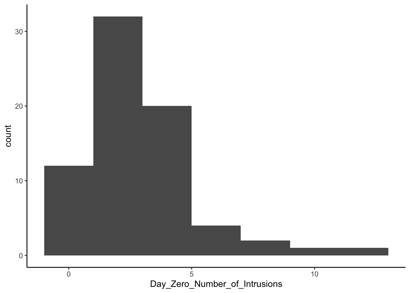
Are these data normal? Close enough, but not terribly normal—probably we don’t need to be concerned in this case, I’d say.
For these Day_Zero_Number_of_Intrustions data, we SHOULD anticipate finding no difference between groups. (Why? Because it’s before the manipulation has happened.) Let’s visualize it first. I’ve plotted the data below. Can you recreate this plot in Jamovi? You should be able to create a similar plot. You may want to scroll back up to the section on conditions to see which number corresponds to which condition. Then, under Data, change each number currently listed as Condition to correctly reflect what condition they are in. (You don’t need to use Transform; just changing the text in Levels should work this time.) After you’ve finished, use Descriptives to plot the boxplots with the data on top.
NoteI forgot how to do this—remind me? (Click to expand)
After loading these data into Jamovi, under the Data tab double click on the Condition variable. Under Levels, change the numbers to text of the conditions above. So:
1will becomeControl2will becomeReactivation+Tetris3will becomeTetris4will becomeReactivation
Now, go to Analyses in the ribbon at the top of the screen, then click on Exploration, and then Descriptives. Put Day_Zero_Number_of_Intrustions into the Variables window, then put Condition into the Split by window.
Under Plots, below, check off Box plot and then check off Data. (Jittered will automatically be selected.) Your plot should now look similar to the below.
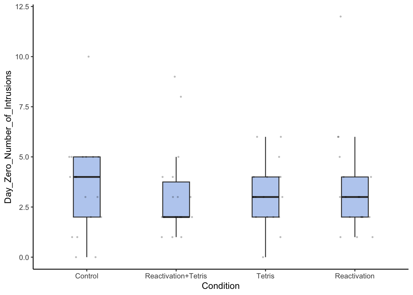
Your plot should have different distribution of the points, which are jittered, but should be quite similar. Export or screenshot the plot you create, and include it in your answer sheet as #1.
Based on this plot, should you expect to see a significant difference between groups? Answer this for #2.
The ANOVA in Jamovi
Run an ANOVA by going to Analyses: ANOVA: One-Way ANOVA. Test what you were looking at in the plot: does condition predict the number of intrusions on Day 0? Turn on the checkbox for Assume Equal (Fisher’s test) and the Descriptives plot. I’ll write up the results for you. Follow this method on other ANOVAs:
There was no significant effect of condition on intrusions on Day 0, \(F(3, 68)=0.16, p=.92\).
If our test had been significant, we would have written \(p<.05\) instead of giving the p-value.
As you’ll note, and as we discussed in class, there are two degrees of freedom: first the between-groups df and then the within-groups df. Like with a t-test, we also report the degrees of freedom. With t-tests, you report something like t(df)=t-value, p < .05 (or \(p=value\)). With an ANOVA, you do the same thing: \(F(\mathit{df_b},\mathit{df_w})=\mathrm{Fvalue}, p<.05\) (or \(p=value\)).
In a more narrative form, I might write:
There was no difference between conditions in the number of intrusions at baseline before the intervention occurred, \(F(3,68)=0.16,p=.92\). Group means varied from \(M=3.17\) intrusions for the Tetris condition to \(M=3.56\) for the control condition, but there was no statistically-significant difference.
What Jamovi gave us here is actually a sort of simplistic version of the ANOVA. It shows us all of the things you need to report as above, but much of the time you’re going to want a bit more: the \(MS_{within}\) and \(MS_{between}\). We’ll calculate these together, then get them from Jamovi.
What’s going on underneath?
To calculate the ANOVA by getting the component parts, we’ll need to get the pieces to find the F ratio. This section might be useful for understanding how to do the calculations we’ve been discussing in class.
I’ll give you the formulae, and then explain getting the mean-squares, and finally the F statistic. You should confirm that you are doing this correctly once you get the \(MS_{within}\) and \(MS_{between}\) from Jamovi directly. Again, we won’t normally be doing all of these calculations, but it’s worth working through this a few times.
- Calculate your degrees of freedom for between and within. \(\mathit{df}_{between}=G-1\) and \(\mathit{df}_{within}=N-G\). Remember that \(N\) is number of participants (total) and \(G\) is number of groups. (Also remember that we just discussed this answer above.) Write these as #3.
Calculate the within-groups mean squares (i.e., variance) in two steps. Remember, \(MS_{within}=\frac{S^2_1+S^2_2+S^2_3+S^2_4}{G}\)—that is, it’s the average of the variances of each group.
- Get the variance of
Day_Zero_Number_of_Intrusionsfor each Condition under Descriptives. (Yes, it will give you variance if you check that checkbox.) - Write those four variances down somewhere. Then, take their average. That is, add them to one another and then divide by 4. This is \(MS_{within}\). Write it as number 4.
- Get the variance of
ImportantYou need to get each group’s variance and then average them—you can’t just get the variance for the entire sample
Calculate the between-groups variance. We need 2 numbers per group, and then one average for the whole… and then we’ll plug them into a formula. I recommend writing each of these down. However, only one of them should be turned in on your answer sheet.
Get the average for the group mean: use the Descriptives menu to get the average of
Day_Zero_Number_of_Intrusionswithout any split by or grouping variable. Label this GM, or Grand Mean.Write down the \(n\) per group and the \(M\) per group. (So, add the split by for
Conditionback in and get the number of participants per group and the means.)Those are our nine numbers: the four \(n\)s, the four \(M\)s, and the \(GM\). Calculate the sum of squares for the between-subjects part of the ANOVA using the following formula: \(SS_{between}=\sum{(n\times{}(M-GM)^2)}\). Essentially, you’re getting the sum of squared deviations but rather than using individual participants’s scores you’re using the group means and subtracting from the grand mean or GM, and then weighting this by the number of participants in each group. For the first one, this is \(18\times{}(3.56-3.32)^2=1.0368\approx{}1.04\). Do the other three, and then sum them up. This is \(SS_{between}\).
Finally, calculate \(MS_{between}\), which is found by \(MS_{between}=\frac{SS_{between}}{df_{between}}\). You got \(SS_{between}\) in c. You got \(df_{between}\) in #3, but also: \(df_{between}=G-1\), where G is the number of groups. Calculate your \(MS_{between}\) from that ratio. Write the \(MS_{between}\) as #5 on your answer sheet.
Now that we have \(MS_{between}\) and \(MS_{within}\), we can find the F statistic, which is the ANOVA’s statistic in the same way that finding t was the main statistic for the t-test. This part is straightforward; it’s a ratio.
\[F=\frac{S_{between}^2}{S_{within}^2}=\frac{MS_{between}}{MS_{within}}\]
So, calculate F with the answers you found in the previous two questions.
You should get the same F-value we previously found from Jamovi and which I reported for you above. Because the between-participants variance is smaller than the within-participants variance, F will be small. In fact, it’s less than 1; any F of 1 or less is clearly not big enough to reject our null. (We’ll discuss how to use an F-table in class, but you don’t need to pull it out here.)
Get the full ANOVA table in Jamovi
Okay, back to doing this fully in Jamovi. Go to Analyses: ANOVA: ANOVA. ( Note: This is not just “One-Way”.) Condition is your fixed factor. Day_Zero_Number_of_Intrusions is still your DV. You should see a table similar to this one:
| Sum of Squares | df | Mean Square | F | p | |
|---|---|---|---|---|---|
| Condition | 2.49 | 3 | 0.829 | 0.163 | 0.921 |
| Residuals | 345.17 | 68 | 5.076 |
Where it says “Condition”, that’s the between-groups row. And where it says “Residuals”—that’s the within-groups bit.
Do the values for \(MS\) and \(F\) match what you calculated? If not, consider revisiting your calculations and figuring out what went wrong.
Do it on your own
Run two ANOVAs: one asking whether
Conditiondetermines the number of intrusive thoughts in the days after the intervention (Days_One_to_Seven_Number_of_Intrusions), and the second asking whetherConditionimpacts the responses on the task that was designed to measure intrusive thoughts (Number_of_Provocation_Task_Intrusions).For each ANOVA, you should report the results as we did in the tutorial—complete with (some of the) means and the \(F(df_1,df_2)=value,p<.05\) or \(p=value\). These are #6a and #6b. Do you understand what these results mean?
For the provocation task test’s results, scroll down in Jamovi under the ANOVA menu and click the drop-down for Estimated Marginal Means. Move
Conditionto Term 1, check off “observed scores” under where it says Plot, and look at the resulting plot. Export/screenshot/copy it into your answer sheet. Then answer: which group(s) are different from the other(s)? This is #7.Under the Data tab, make sure that
Number_of_Provocation_Task_Intrusionsis a continuous variable. (It may not have been imported as one.) Then, under Analyses: Exploration: Descriptives: Plots, make a bar plot (not a box plot) showingNumber_of_Provocation_Task_Intrusionssplit byCondition. Export/screenshot/copy this plot to your answer sheet. Which plot (this or #7) do you prefer? These two answers are #8.
Pairwise tests
I told you in class that you shouldn’t repeatedly use t-tests because of the fact that doing such multiple comparisons increases your Type I error rate (i.e., risk of false positives). However, you can do what are called planned comparisons. After a significant result on an ANOVA, you may compare the condition of interest against the others if you intended to do so before starting. (This is one more reason why preregistration is so important!) Usually, even when you’ve planned to do comparisons, you should do a correction for the planned comparison. In this case, we want to compare the Reactivation + Tetris condition to the others. (This was the one we hoped would work.) We don’t need to make every other comparison.
In your ANOVA menu, you can do this easily. Let’s stick to the previous ANOVA looking at the provocation task. Scroll down to where it says “Post-hoc tests” and open the menu. Put Condition in the right side of the test window. Make sure “Tukey” is checked ON under Correction (and “No correction” is not checked). Check ON the Cohen’s d for Effect Size as well. In the results, you’ll see a few corrected t-test values for each possible (pairwise) comparison. The final column is the corrected p-value; the penultimate is the t-value. Pick one that’s statistically significant (i.e., where \(p<.05\)) based on the Tukey-corrected p-value.
- For #9, write up the results of the significant post-hoc t-test, just using what Jamovi gave you.
Then, under Data, filter to just those two conditions. Remember that you need to repeat the variable name (Condition) each time you set it == to the condition names. Remember, too, that spelling, capitalization, and spacing all matter.
NoteI forgot how to do this—remind me? (Click to expand)
Under the Data menu, click Filters. Under the first one (Filter 1), click into the textbox next to where it says \(f_x=\) and type: Condition == "Control" or Condition == "Tetris", but replace the names Control and Tetris with whichever groups you want to focus on. Make sure to use quotation marks and the double equal signs, and to repeat the name of the variable (Condition) for each time you use it.
- Once the filter is working for just two conditions, run an independent-samples t-test predicting
Number_of_Provocation_Task_IntrusionsbyCondition. For #10, write up these results, and then answer: what (if anything) is different in this non-corrected result?
That’s it.
Reuse
Citation
BibTeX citation:
@online{dainer-best2025,
  author = {Dainer-Best, Justin},
  title = {One-Way {ANOVA} {(Lab} 9)},
  date = {2025-10-30},
  url = {https://faculty.bard.edu/jdainerbest/stats/labs/posts/09-one-way-anova/},
  langid = {en}
}
For attribution, please cite this work as:
Dainer-Best, Justin. 2025. “One-Way ANOVA (Lab 9).” October
30, 2025. https://faculty.bard.edu/jdainerbest/stats/labs/posts/09-one-way-anova/.