
Today’s lab is focused on these objectives:
- Learning how to implement a basic hypothesis test in Jamovi
- Practicing the data visualization skills you learned in the previous lab
You’ll turn in an “answer sheet” on Brightspace. Please be sure to turn that in by the end of the weekend. Note that there is no lab next week!
In today’s lab, we’re using data from a small sample and pretending it’s from a population. That’s fine, because we’re learning here—but in the future, you should not use a z-test to run analyses.
Friends questions
Today, we’ll be using your friends data for a few simple questions:
- Would someone who was 6’5” be considered to have a “significantly different” height among Bard students?
- Would they be considered “significantly tall” compared to other Bard students?
- Would someone who doesn’t watch any TV be considered a statistically-significant outlier among Bard students?
- Would that person be considered to watch significantly less TV than other Bard students?
You’ll note that (2) and (4) are research questions about which we can develop one-tailed hypotheses.
Steps of hypothesis-testing
Step 1
Step 1: Restate question as a research and null hypothesis
We asked: Would someone who was 6’5” be considered to have a “significantly different” height among Bard students? Read the questions below. I’ve answered them for you—you should click the question to see the answer.
What is the framing of this for the research hypothesis?
People who are as tall as this person are different from Bard students as a whole
What is the framing of this for the null hypothesis?
People who are as tall as this person are no different from Bard students as a whole
Ultimately, we’re interested in means, as you’ll remember—the statistical framing of these hypotheses. How do the means of people like this person compare to the means of students at Bard. We can frame the research hypothesis as: \(\mu_{\mathrm{Bard~students~of~this~height}}\neq\mu_{\mathrm{Bard~students~in~general}}\) and the null hypothesis as: \(\mu_{\mathrm{Bard~students~of~this~height}}=\mu_{\mathrm{Bard~students~in~general}}\)
Steps 2 and 3
Step 2: Determine the characteristics of the comparison distribution
Step 3: Determine the sample cutoff score to reject the null hypothesis
In this case, we’re continuing to use the distribution of z-scores.
Which of the following is/are true about a z-score distribution?
- We assume that it is normally-distributed
- It has a mean of 0
- It has a standard deviation of 1
- It is symmetrical
See the answer.
They are all true.
What is the cut-off score for the z-distribution when using a cutoff of p = .05?
The cut-off is \(\pm{}1.96\).
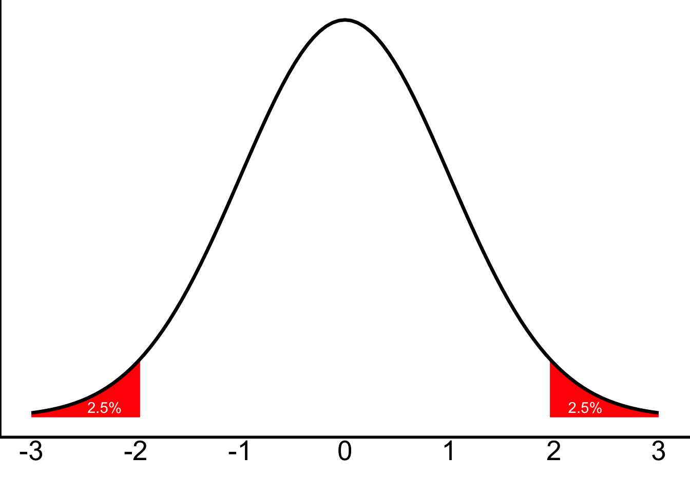
Remember how in class we discussed the fact that what we actually want to get the most extreme 5% of scores is the bottom 2.5% of scores and the top 2.5% of scores? Something like this:
Well, we can also think of those as cut-offs for the lowest 2.5% of scores and the highest 2.5% of scores—something like this. (The 97.5% is just 100% - 2.5%.)
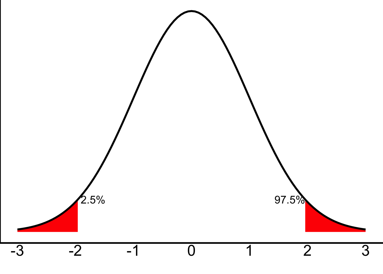
That is to say: if there’s 2.5% in each tail, then on the left side, 2.5% of scores are in that left, red tail. On the right side, 97.5% of scores will fall before the right, red tail.
Okay! With those two questions, we’ve gotten through Steps 2 and 3 for the first research question!
Step 4: Determine your sample’s score
Now, we haven’t played with our data yet. The information on heights is saved in the data-frame friends. The friends dataset is available on Brightspace, here, or for download here. I’ve edited it slightly at this point. It should be a bit easier to work with!
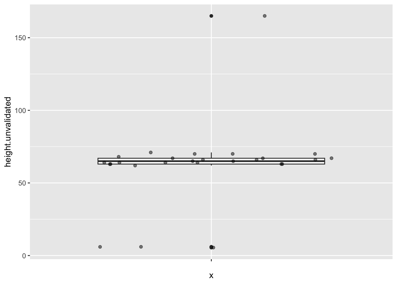
Load the friends data into Jamovi. Find the range and mean of the variable height.unvalidated. If you’ve loaded it correctly, you should see the mean as 62.7 and the range as 5.5, 165. You might note that the range doesn’t make much sense. I’ll tell you why: we asked for height, in inches, but someone seems to have given height in feet. That’s why the variable is called “unvalidated”; in Qualtrics we could have thrown an error there, but we chose not to.
You could also have caught this if you make a box plot:
Find the three people who gave their height in feet, and (manually, probably) correct them to be in inches. Remember, 1 foot = 12 inches.
But there’s also no way that someone is 165 inches tall! We have two choices here: remove this participant or assume that they answered with the height in centimeters. I’d suggest you assume the latter. Correct this person’s answer as well, assuming that there are 2.54 cm in 1 in. (You can round to 2 decimals.)
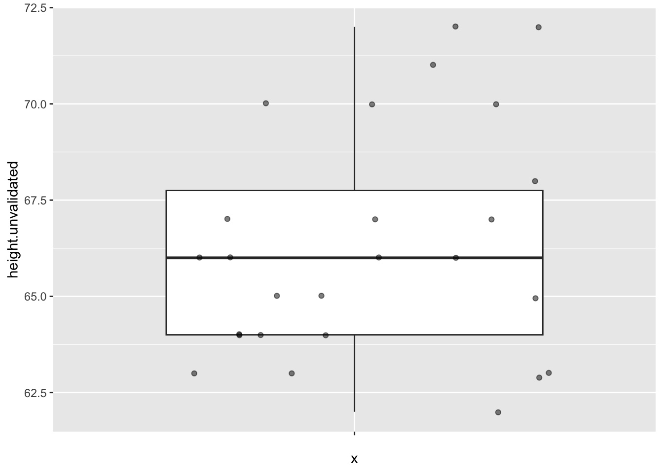
Then find the mean, range, and standard deviation. This is question #1 on your answer sheet.
Your boxplot should look better now:
We now need to complete Step 4 and determine the z-score. We know how to determine a z-score already. Let’s do it. Remember that \(z=\frac{X-M}{SD}\) or (in population terms) \(z=\frac{X-\mu}{\sigma}\). So our sample—from which we’ll estimate the mean and standard deviation—will be students in this survey. You’ll see soon enough that we normally make corrections for the fact that this is only an estimate… but for today, let’s just make use of the means and standard deviations of the height in Jamovi. You should have gotten those in the same step where you found the range and mean.
Our research question is this: Would someone who was 6’5” be considered to have a “significantly different” height among Bard students? Well, now we can get the z-score for that person. Convert 6’5” to inches. Since \(z=(X-M)/SD\), we can fill this in from what we have. Solve for z; I recommend just doing it on paper. This is answer #2.
Step 5: Decide whether or not to reject the null hypothesis
Just by looking at your z-score, you should have an idea of whether or not we’ll reject the null. As we discussed in Steps 2 and 3, our cut-off is \(\pm1.96\).
Based on the z-score and the cutoff above, should we reject the null hypothesis?
Yes, because the z-score is higher than our cutoff. We can reject the null hypothesis—that there is no difference between this score and the population.
We can simply compare this score to our cutoff—is it more than \(+1.96\) or less than \(-1.96\)? It is larger than 1.96.
In this case, it’s actually a lot bigger. 99.98% of scores are lower than this one. Having a height of 6’5” in our sample would be extremely unlikely—such a person would fall in the top 99.98% of the sample.
Compare to a z-table (where we would need to add 50% to the “% Mean to z” column or subtract the “% in Tail” column from 100%). (Scroll down to get to the z we’ve found.)
| z | % Mean to z | % in Tail |
|---|---|---|
| 0.00 | 0.00 | 50.00 |
| 0.01 | 0.40 | 49.60 |
| 0.02 | 0.80 | 49.20 |
| 0.03 | 1.20 | 48.80 |
| 0.04 | 1.60 | 48.40 |
| 0.05 | 1.99 | 48.01 |
| 0.06 | 2.39 | 47.61 |
| 0.07 | 2.79 | 47.21 |
| 0.08 | 3.19 | 46.81 |
| 0.09 | 3.59 | 46.41 |
| 0.10 | 3.98 | 46.02 |
| 0.11 | 4.38 | 45.62 |
| 0.12 | 4.78 | 45.22 |
| 0.13 | 5.17 | 44.83 |
| 0.14 | 5.57 | 44.43 |
| 0.15 | 5.96 | 44.04 |
| 0.16 | 6.36 | 43.64 |
| 0.17 | 6.75 | 43.25 |
| 0.18 | 7.14 | 42.86 |
| 0.19 | 7.53 | 42.47 |
| 0.20 | 7.93 | 42.07 |
| 0.21 | 8.32 | 41.68 |
| 0.22 | 8.71 | 41.29 |
| 0.23 | 9.10 | 40.90 |
| 0.24 | 9.48 | 40.52 |
| 0.25 | 9.87 | 40.13 |
| 0.26 | 10.26 | 39.74 |
| 0.27 | 10.64 | 39.36 |
| 0.28 | 11.03 | 38.97 |
| 0.29 | 11.41 | 38.59 |
| 0.30 | 11.79 | 38.21 |
| 0.31 | 12.17 | 37.83 |
| 0.32 | 12.55 | 37.45 |
| 0.33 | 12.93 | 37.07 |
| 0.34 | 13.31 | 36.69 |
| 0.35 | 13.68 | 36.32 |
| 0.36 | 14.06 | 35.94 |
| 0.37 | 14.43 | 35.57 |
| 0.38 | 14.80 | 35.20 |
| 0.39 | 15.17 | 34.83 |
| 0.40 | 15.54 | 34.46 |
| 0.41 | 15.91 | 34.09 |
| 0.42 | 16.28 | 33.72 |
| 0.43 | 16.64 | 33.36 |
| 0.44 | 17.00 | 33.00 |
| 0.45 | 17.36 | 32.64 |
| 0.46 | 17.72 | 32.28 |
| 0.47 | 18.08 | 31.92 |
| 0.48 | 18.44 | 31.56 |
| 0.49 | 18.79 | 31.21 |
| 0.50 | 19.15 | 30.85 |
| 0.51 | 19.50 | 30.50 |
| 0.52 | 19.85 | 30.15 |
| 0.53 | 20.19 | 29.81 |
| 0.54 | 20.54 | 29.46 |
| 0.55 | 20.88 | 29.12 |
| 0.56 | 21.23 | 28.77 |
| 0.57 | 21.57 | 28.43 |
| 0.58 | 21.90 | 28.10 |
| 0.59 | 22.24 | 27.76 |
| 0.60 | 22.57 | 27.43 |
| 0.61 | 22.91 | 27.09 |
| 0.62 | 23.24 | 26.76 |
| 0.63 | 23.57 | 26.43 |
| 0.64 | 23.89 | 26.11 |
| 0.65 | 24.22 | 25.78 |
| 0.66 | 24.54 | 25.46 |
| 0.67 | 24.86 | 25.14 |
| 0.68 | 25.17 | 24.83 |
| 0.69 | 25.49 | 24.51 |
| 0.70 | 25.80 | 24.20 |
| 0.71 | 26.11 | 23.89 |
| 0.72 | 26.42 | 23.58 |
| 0.73 | 26.73 | 23.27 |
| 0.74 | 27.04 | 22.96 |
| 0.75 | 27.34 | 22.66 |
| 0.76 | 27.64 | 22.36 |
| 0.77 | 27.94 | 22.06 |
| 0.78 | 28.23 | 21.77 |
| 0.79 | 28.52 | 21.48 |
| 0.80 | 28.81 | 21.19 |
| 0.81 | 29.10 | 20.90 |
| 0.82 | 29.39 | 20.61 |
| 0.83 | 29.67 | 20.33 |
| 0.84 | 29.95 | 20.05 |
| 0.85 | 30.23 | 19.77 |
| 0.86 | 30.51 | 19.49 |
| 0.87 | 30.78 | 19.22 |
| 0.88 | 31.06 | 18.94 |
| 0.89 | 31.33 | 18.67 |
| 0.90 | 31.59 | 18.41 |
| 0.91 | 31.86 | 18.14 |
| 0.92 | 32.12 | 17.88 |
| 0.93 | 32.38 | 17.62 |
| 0.94 | 32.64 | 17.36 |
| 0.95 | 32.89 | 17.11 |
| 0.96 | 33.15 | 16.85 |
| 0.97 | 33.40 | 16.60 |
| 0.98 | 33.65 | 16.35 |
| 0.99 | 33.89 | 16.11 |
| 1.00 | 34.13 | 15.87 |
| 1.01 | 34.38 | 15.62 |
| 1.02 | 34.61 | 15.39 |
| 1.03 | 34.85 | 15.15 |
| 1.04 | 35.08 | 14.92 |
| 1.05 | 35.31 | 14.69 |
| 1.06 | 35.54 | 14.46 |
| 1.07 | 35.77 | 14.23 |
| 1.08 | 35.99 | 14.01 |
| 1.09 | 36.21 | 13.79 |
| 1.10 | 36.43 | 13.57 |
| 1.11 | 36.65 | 13.35 |
| 1.12 | 36.86 | 13.14 |
| 1.13 | 37.08 | 12.92 |
| 1.14 | 37.29 | 12.71 |
| 1.15 | 37.49 | 12.51 |
| 1.16 | 37.70 | 12.30 |
| 1.17 | 37.90 | 12.10 |
| 1.18 | 38.10 | 11.90 |
| 1.19 | 38.30 | 11.70 |
| 1.20 | 38.49 | 11.51 |
| 1.21 | 38.69 | 11.31 |
| 1.22 | 38.88 | 11.12 |
| 1.23 | 39.07 | 10.93 |
| 1.24 | 39.25 | 10.75 |
| 1.25 | 39.44 | 10.56 |
| 1.26 | 39.62 | 10.38 |
| 1.27 | 39.80 | 10.20 |
| 1.28 | 39.97 | 10.03 |
| 1.29 | 40.15 | 9.85 |
| 1.30 | 40.32 | 9.68 |
| 1.31 | 40.49 | 9.51 |
| 1.32 | 40.66 | 9.34 |
| 1.33 | 40.82 | 9.18 |
| 1.34 | 40.99 | 9.01 |
| 1.35 | 41.15 | 8.85 |
| 1.36 | 41.31 | 8.69 |
| 1.37 | 41.47 | 8.53 |
| 1.38 | 41.62 | 8.38 |
| 1.39 | 41.77 | 8.23 |
| 1.40 | 41.92 | 8.08 |
| 1.41 | 42.07 | 7.93 |
| 1.42 | 42.22 | 7.78 |
| 1.43 | 42.36 | 7.64 |
| 1.44 | 42.51 | 7.49 |
| 1.45 | 42.65 | 7.35 |
| 1.46 | 42.79 | 7.21 |
| 1.47 | 42.92 | 7.08 |
| 1.48 | 43.06 | 6.94 |
| 1.49 | 43.19 | 6.81 |
| 1.50 | 43.32 | 6.68 |
| 1.51 | 43.45 | 6.55 |
| 1.52 | 43.57 | 6.43 |
| 1.53 | 43.70 | 6.30 |
| 1.54 | 43.82 | 6.18 |
| 1.55 | 43.94 | 6.06 |
| 1.56 | 44.06 | 5.94 |
| 1.57 | 44.18 | 5.82 |
| 1.58 | 44.29 | 5.71 |
| 1.59 | 44.41 | 5.59 |
| 1.60 | 44.52 | 5.48 |
| 1.61 | 44.63 | 5.37 |
| 1.62 | 44.74 | 5.26 |
| 1.63 | 44.84 | 5.16 |
| 1.64 | 44.95 | 5.05 |
| 1.65 | 45.05 | 4.95 |
| 1.66 | 45.15 | 4.85 |
| 1.67 | 45.25 | 4.75 |
| 1.68 | 45.35 | 4.65 |
| 1.69 | 45.45 | 4.55 |
| 1.70 | 45.54 | 4.46 |
| 1.71 | 45.64 | 4.36 |
| 1.72 | 45.73 | 4.27 |
| 1.73 | 45.82 | 4.18 |
| 1.74 | 45.91 | 4.09 |
| 1.75 | 45.99 | 4.01 |
| 1.76 | 46.08 | 3.92 |
| 1.77 | 46.16 | 3.84 |
| 1.78 | 46.25 | 3.75 |
| 1.79 | 46.33 | 3.67 |
| 1.80 | 46.41 | 3.59 |
| 1.81 | 46.49 | 3.51 |
| 1.82 | 46.56 | 3.44 |
| 1.83 | 46.64 | 3.36 |
| 1.84 | 46.71 | 3.29 |
| 1.85 | 46.78 | 3.22 |
| 1.86 | 46.86 | 3.14 |
| 1.87 | 46.93 | 3.07 |
| 1.88 | 46.99 | 3.01 |
| 1.89 | 47.06 | 2.94 |
| 1.90 | 47.13 | 2.87 |
| 1.91 | 47.19 | 2.81 |
| 1.92 | 47.26 | 2.74 |
| 1.93 | 47.32 | 2.68 |
| 1.94 | 47.38 | 2.62 |
| 1.95 | 47.44 | 2.56 |
| 1.96 | 47.50 | 2.50 |
| 1.97 | 47.56 | 2.44 |
| 1.98 | 47.61 | 2.39 |
| 1.99 | 47.67 | 2.33 |
| 2.00 | 47.72 | 2.28 |
| 2.01 | 47.78 | 2.22 |
| 2.02 | 47.83 | 2.17 |
| 2.03 | 47.88 | 2.12 |
| 2.04 | 47.93 | 2.07 |
| 2.05 | 47.98 | 2.02 |
| 2.06 | 48.03 | 1.97 |
| 2.07 | 48.08 | 1.92 |
| 2.08 | 48.12 | 1.88 |
| 2.09 | 48.17 | 1.83 |
| 2.10 | 48.21 | 1.79 |
| 2.11 | 48.26 | 1.74 |
| 2.12 | 48.30 | 1.70 |
| 2.13 | 48.34 | 1.66 |
| 2.14 | 48.38 | 1.62 |
| 2.15 | 48.42 | 1.58 |
| 2.16 | 48.46 | 1.54 |
| 2.17 | 48.50 | 1.50 |
| 2.18 | 48.54 | 1.46 |
| 2.19 | 48.57 | 1.43 |
| 2.20 | 48.61 | 1.39 |
| 2.21 | 48.64 | 1.36 |
| 2.22 | 48.68 | 1.32 |
| 2.23 | 48.71 | 1.29 |
| 2.24 | 48.75 | 1.25 |
| 2.25 | 48.78 | 1.22 |
| 2.26 | 48.81 | 1.19 |
| 2.27 | 48.84 | 1.16 |
| 2.28 | 48.87 | 1.13 |
| 2.29 | 48.90 | 1.10 |
| 2.30 | 48.93 | 1.07 |
| 2.31 | 48.96 | 1.04 |
| 2.32 | 48.98 | 1.02 |
| 2.33 | 49.01 | 0.99 |
| 2.34 | 49.04 | 0.96 |
| 2.35 | 49.06 | 0.94 |
| 2.36 | 49.09 | 0.91 |
| 2.37 | 49.11 | 0.89 |
| 2.38 | 49.13 | 0.87 |
| 2.39 | 49.16 | 0.84 |
| 2.40 | 49.18 | 0.82 |
| 2.41 | 49.20 | 0.80 |
| 2.42 | 49.22 | 0.78 |
| 2.43 | 49.25 | 0.75 |
| 2.44 | 49.27 | 0.73 |
| 2.45 | 49.29 | 0.71 |
| 2.46 | 49.31 | 0.69 |
| 2.47 | 49.32 | 0.68 |
| 2.48 | 49.34 | 0.66 |
| 2.49 | 49.36 | 0.64 |
| 2.50 | 49.38 | 0.62 |
| 2.51 | 49.40 | 0.60 |
| 2.52 | 49.41 | 0.59 |
| 2.53 | 49.43 | 0.57 |
| 2.54 | 49.45 | 0.55 |
| 2.55 | 49.46 | 0.54 |
| 2.56 | 49.48 | 0.52 |
| 2.57 | 49.49 | 0.51 |
| 2.58 | 49.51 | 0.49 |
| 2.59 | 49.52 | 0.48 |
| 2.60 | 49.53 | 0.47 |
| 2.61 | 49.55 | 0.45 |
| 2.62 | 49.56 | 0.44 |
| 2.63 | 49.57 | 0.43 |
| 2.64 | 49.59 | 0.41 |
| 2.65 | 49.60 | 0.40 |
| 2.66 | 49.61 | 0.39 |
| 2.67 | 49.62 | 0.38 |
| 2.68 | 49.63 | 0.37 |
| 2.69 | 49.64 | 0.36 |
| 2.70 | 49.65 | 0.35 |
| 2.71 | 49.66 | 0.34 |
| 2.72 | 49.67 | 0.33 |
| 2.73 | 49.68 | 0.32 |
| 2.74 | 49.69 | 0.31 |
| 2.75 | 49.70 | 0.30 |
| 2.76 | 49.71 | 0.29 |
| 2.77 | 49.72 | 0.28 |
| 2.78 | 49.73 | 0.27 |
| 2.79 | 49.74 | 0.26 |
| 2.80 | 49.74 | 0.26 |
| 2.81 | 49.75 | 0.25 |
| 2.82 | 49.76 | 0.24 |
| 2.83 | 49.77 | 0.23 |
| 2.84 | 49.77 | 0.23 |
| 2.85 | 49.78 | 0.22 |
| 2.86 | 49.79 | 0.21 |
| 2.87 | 49.79 | 0.21 |
| 2.88 | 49.80 | 0.20 |
| 2.89 | 49.81 | 0.19 |
| 2.90 | 49.81 | 0.19 |
| 2.91 | 49.82 | 0.18 |
| 2.92 | 49.82 | 0.18 |
| 2.93 | 49.83 | 0.17 |
| 2.94 | 49.84 | 0.16 |
| 2.95 | 49.84 | 0.16 |
| 2.96 | 49.85 | 0.15 |
| 2.97 | 49.85 | 0.15 |
| 2.98 | 49.86 | 0.14 |
| 2.99 | 49.86 | 0.14 |
| 3.00 | 49.87 | 0.13 |
| 3.01 | 49.87 | 0.13 |
| 3.02 | 49.87 | 0.13 |
| 3.03 | 49.88 | 0.12 |
| 3.04 | 49.88 | 0.12 |
| 3.05 | 49.89 | 0.11 |
| 3.06 | 49.89 | 0.11 |
| 3.07 | 49.89 | 0.11 |
| 3.08 | 49.90 | 0.10 |
| 3.09 | 49.90 | 0.10 |
| 3.10 | 49.90 | 0.10 |
| 3.11 | 49.91 | 0.09 |
| 3.12 | 49.91 | 0.09 |
| 3.13 | 49.91 | 0.09 |
| 3.14 | 49.92 | 0.08 |
| 3.15 | 49.92 | 0.08 |
| 3.16 | 49.92 | 0.08 |
| 3.17 | 49.92 | 0.08 |
| 3.18 | 49.93 | 0.07 |
| 3.19 | 49.93 | 0.07 |
| 3.20 | 49.93 | 0.07 |
| 3.21 | 49.93 | 0.07 |
| 3.22 | 49.94 | 0.06 |
| 3.23 | 49.94 | 0.06 |
| 3.24 | 49.94 | 0.06 |
| 3.25 | 49.94 | 0.06 |
| 3.26 | 49.94 | 0.06 |
| 3.27 | 49.95 | 0.05 |
| 3.28 | 49.95 | 0.05 |
| 3.29 | 49.95 | 0.05 |
| 3.30 | 49.95 | 0.05 |
| 3.31 | 49.95 | 0.05 |
| 3.32 | 49.95 | 0.05 |
| 3.33 | 49.96 | 0.04 |
| 3.34 | 49.96 | 0.04 |
| 3.35 | 49.96 | 0.04 |
| 3.36 | 49.96 | 0.04 |
| 3.37 | 49.96 | 0.04 |
| 3.38 | 49.96 | 0.04 |
| 3.39 | 49.97 | 0.03 |
| 3.40 | 49.97 | 0.03 |
| 3.41 | 49.97 | 0.03 |
| 3.42 | 49.97 | 0.03 |
| 3.43 | 49.97 | 0.03 |
| 3.44 | 49.97 | 0.03 |
| 3.45 | 49.97 | 0.03 |
| 3.46 | 49.97 | 0.03 |
| 3.47 | 49.97 | 0.03 |
| 3.48 | 49.97 | 0.03 |
| 3.49 | 49.98 | 0.02 |
| 3.50 | 49.98 | 0.02 |
| 3.51 | 49.98 | 0.02 |
| 3.52 | 49.98 | 0.02 |
| 3.53 | 49.98 | 0.02 |
| 3.54 | 49.98 | 0.02 |
| 3.55 | 49.98 | 0.02 |
| 3.56 | 49.98 | 0.02 |
| 3.57 | 49.98 | 0.02 |
| 3.58 | 49.98 | 0.02 |
| 3.59 | 49.98 | 0.02 |
| 3.60 | 49.98 | 0.02 |
| 3.61 | 49.98 | 0.02 |
| 3.62 | 49.99 | 0.01 |
| 3.63 | 49.99 | 0.01 |
| 3.64 | 49.99 | 0.01 |
| 3.65 | 49.99 | 0.01 |
A one-tailed test
We can do this again as a one-tailed test much more quickly now that we have the basics! Let’s take the same person—6’5” in height—and return to this question: Would they be considered “significantly tall” compared to other Bard students? Imagine in this case that we don’t care whether they’re on the short side.
Step 1: Restate question as a research and null hypothesis
We can reframe the research hypothesis as “People who are as tall as this person are taller than Bard students as a whole” and the null as “People who are as tall as this person are the same height or shorter than Bard students as a whole”.
We can frame the research hypothesis in statistical terms as \(\mu_{\mathrm{Bard~students~of~this~height}}>\mu_{\mathrm{Bard~students~in~general}}\) and the null hypothesis as \(\mu_{\mathrm{Bard~students~of~this~height}}\leq\mu_{\mathrm{Bard~students~in~general}}\)
Remember, that it’s not just LESS THAN—it’s LESS THAN OR EQUAL TO.
Steps 2 and 3
Step 2: Determine the characteristics of the comparison distribution
Step 3: Determine the sample cutoff score to reject the null hypothesis
We’re still using the z-distribution, but now we’re only interested in scores that fall in the upper 5% of the distribution—where 95% of the scores fall below:
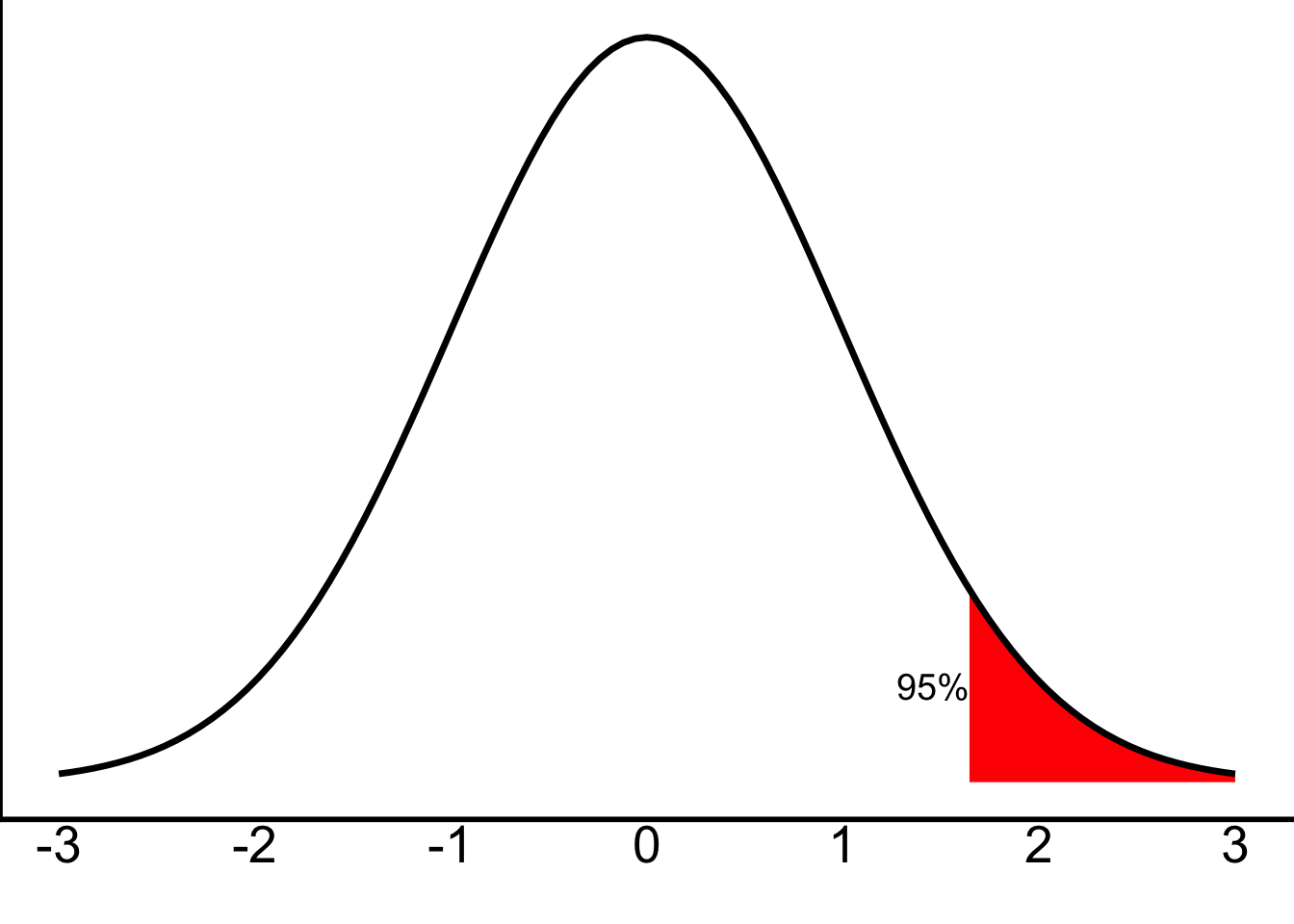
And just as we discussed in class, our lower cut-off will be \(+1.64\). Any z-score above that will be “unlikely” and let us know that \(p<.05\). Why 1.64 instead of 1.96? Well, 1.96 corresponded to 2.5% in either tail (i.e., a total of 5%), whereas 1.64 corresponds to 5% just in one tail. Feel free to scroll up to the z-table in the note above to confirm that.
Step 4: Determine your sample’s score
You already determined the score! You indicated it in answer #2; it’s the z-score for the person with a height of 6’5”.
Step 5: Decide whether or not to reject the null hypothesis
To decide whether or not to reject the null hypothesis, we have an easy starting point: if something was statistically significant for a two-tailed test, a one-tailed test will always be statistically significant at the same p-value. (One-tailed tests, as we discussed in class, can be “more lenient”, because they’re only “looking” at one tail of the distribution.)
But, just in case, here we can simply compare to our cutoff of \(+1.64\).
And reject the null. We have evidence that this person is taller than most other Bard students.
Trying this out a bit more
Above, I have walked you through these steps. Let’s do a bit more on your own.
The questions I described above were:
Would someone who doesn’t watch any TV be considered a statistically-significant outlier among Bard students?
Would that person be considered to watch significantly less TV than other Bard students?
Use the variable tvhours for this. “Not watching any TV [or streaming]” is a 0 on that variable. For #3 on your answer sheet, walk through the five steps of hypothesis-testing using (in #3) a two-tailed test. Then, for #4, do the same thing for the one-tailed test. For each, include a description of what the finding means. What can you conclude?
You may want to include a box plot of your data, to make sure your data seems reasonable (and not to have bizarre outliers).
Extension exercise
If you have more time, want to practice, or are just interested, this is another exercise of the same vein; we may return to this data.
This is a summary of data from Pro Publica, an investigative journalism organization. You can read more about the data here: https://www.propublica.org/article/so-sue-them-what-weve-learned-about-the-debt-collection-lawsuit-machine
| Type | Mean | SD |
|---|---|---|
| Auto | 109.52 | 236.87 |
| Collection Agency | 39.26 | 93.39 |
| Debt Buyer | 316.98 | 867.30 |
| Government | 121.04 | 190.46 |
| High-Cost Lender | 46.00 | 53.49 |
| Insurance | 128.13 | 218.79 |
| Major Bank | 690.02 | 1440.31 |
| Medical | 0.51 | 8.91 |
| Misc | 36.92 | 56.82 |
| Misc Lender | 69.80 | 158.43 |
| Other | 23319.00 | 5151.45 |
| Utility | 53.14 | 55.50 |
Essentially, these data show how often (over 13 years from 2001-2014) the owners of individuals’ debt in Miami-Dade County, Fl sued those individuals. It’s sorted by type of debt.
Your task: In 2000, debt buyers (firms that buy debt to collect) sued individuals 59.8 times. This is your x. Follow the steps of hypothesis-testing to determine whether this is significantly different from the norm over the subsequent 13 years (i.e., from 2001 through 2014), using a z-test and the above information. (You only need to consider the row for debt buyers.) This time, use a cut-off of \(p=.01\), so there is only a significant difference if \(p<.01\).
If you do this, include it as #5 in your answers.
Reuse
Citation
BibTeX citation:
@online{dainer-best2023,
  author = {Dainer-Best, Justin},
  title = {Hypothesis {Testing} {(Lab} 4)},
  date = {2023-09-28},
  url = {https://faculty.bard.edu/jdainerbest/stats/labs//posts/04-hypothesis-testing},
  langid = {en}
}
For attribution, please cite this work as:
Dainer-Best, Justin. 2023. “Hypothesis Testing (Lab 4).”
September 28, 2023. https://faculty.bard.edu/jdainerbest/stats/labs//posts/04-hypothesis-testing.