
| id | hrsd.pre | hrsd.post | hars.pre | hars.post | num.sessions |
|---|---|---|---|---|---|
| P003 | 16 | 3 | 15 | 4 | 9 |
| P004 | 16 | 7 | 33 | 13 | 12 |
| P006 | 13 | 8 | 13 | 6 | 11 |
| P007 | 11 | 3 | 17 | 4 | 14 |
| P009 | 17 | 7 | 9 | 11 | 12 |
| P012 | 9 | 0 | 13 | 1 | 8 |
| P013 | 14 | 3 | 19 | 6 | 10 |
| P014 | 10 | 3 | 12 | 6 | 9 |
| P019 | 10 | 5 | 10 | 3 | 7 |
| P023 | 8 | 1 | 7 | 2 | 10 |
| P040 | 21 | 8 | 41 | 9 | 13 |
| P048 | 14 | 6 | 17 | 8 | 11 |
| P068 | 11 | 6 | 14 | 12 | 9 |
| P072 | 15 | 6 | 13 | 4 | 8 |
| P074 | 12 | 8 | 10 | 11 | 10 |
| P075 | 18 | 11 | 23 | 18 | 8 |
| P100 | 7 | 2 | 14 | 1 | 4 |
| P111 | 18 | 11 | 15 | 8 | 13 |
| P115 | 18 | 8 | 19 | 8 | 9 |
| P117 | 12 | 9 | 18 | 7 | 8 |
| P127 | 9 | 4 | 13 | 5 | 12 |
| P139 | 14 | 9 | 12 | 9 | 14 |
| P160 | 13 | 6 | 11 | 3 | 13 |
| P163 | 16 | 10 | 16 | 5 | 14 |
| P169 | 13 | 9 | 15 | 3 | 12 |
| P202 | 10 | 4 | 11 | 7 | 12 |
| P203 | 18 | 5 | 20 | 10 | 10 |
| P206 | 11 | 2 | 16 | 4 | 9 |
| P219 | 21 | 5 | 27 | 9 | 10 |
| P220 | 14 | 10 | 13 | 9 | 12 |
| P223 | 21 | 3 | 12 | 2 | 9 |
| P244 | 12 | 3 | 8 | 3 | 10 |
Objectives
Today’s lab’s objectives are to:
- Learn about dependent-samples t-tests
- Learn how to conduct independent- and dependent-samples t-tests in Jamovi (and, a little bit, with the help of Jamovi)
- Visualize the results of such tests
You’ll turn in an “answer sheet” on Brightspace. Please be sure to turn that in by the end of the weekend.
Dependent means t-tests
In a dependent means t-test, otherwise-known-as the t-test for dependent means or paired-samples t-test, we are comparing two means that are dependent on one another in some way. The scores are related to one another in a way that’s relatively easy to see—usually, e.g., because it’s the same person who’s doing something at two time-points.
As with the independent-samples t-test, the population’s mean and variance are unknown, and so must be estimated.
In the dependent-samples t-test, we can calculate difference scores with individuals because there is an obvious individual to subtract from—themself—and so we can easily do so. Rather than needing to use a distribution of the differences between means, we can use a single comparison distribution based on those difference scores.
Answer the following questions for yourself before clicking on them to see the answers. I recommend discussing with a neighbor.
Which is the comparison distribution for the t-test for dependent means?
The comparison distribution is a t distribution with a mean of 0 and SD of \(S_M\)
Why is the df in a t-test for dependent means equal to n-1?
Because the paired samples mean that there’s more room for variation – only one of the sample scores needs to be constrained, while all of the others are “free to vary”.
What is the formula for t in the t-test for dependent means?
\[t=\frac{M-\mu}{S_M}\]
It’s the same formula as for the one-sample t-test
Key ideas
So, the major takeaways here are:
The dependent-samples t-test is based on the difference scores, but because those difference scores are calculated within paired participants, the comparison distribution is the sample of those difference scores (rather than needing to only compare the distribution of the difference between the means, as in an independent-samples t-test).
Therefore, this test has \(df=n-1\), like the one-sample t-test, and not \(df=n-2\), like in the t-test for independent means.
The comparison distribution in the dependent-samples t-test is a t distribution with a mean of 0, \(df=n-1\), and a standard deviation based on the distribution of difference scores which is based on that combined distribution’s own \(SD\) and \(n\) (\(S_M=\frac{S}{\sqrt{n}}\)). No pooling is necessary because we treat this as a single distribution.
The cutoff for the sample is based on those degrees of freedom, e.g., -2.78, 2.78 for \(df=4\).
The equation for t has not substantially changed: \(t=\frac{M-\mu}{S_M}\)—and in fact, \(\mu\) in the dependent-samples t-test is always actually equal to 0, because we are always testing whether there is a substantial change from 0.
I’ve suggested that it’s quite easy to identify whether a test should require a t-test for dependent means, or not—because the test obviously includes paired samples. Let’s give it a try. For each of the following, select which kind of test is best. Again, I’d encourage you to discuss with a classmate as you do this.
A researcher wants to test whether the average score on a certain exam taken by college students is different from the average score on the same exam when taken by the general population. The population standard deviation of is known. What type of test should the researcher use?
This is a z-test for a sample. We know something about the ‘average’ person (i.e., the population mean), and want to compare a sample to them. We also know the population standard deviation, so can use a z-test.
A researcher wants to test whether a new drug is effective in reducing anxiety levels. The researcher randomly assigns participants to either receive the new drug or a placebo. What type of test should the researcher use to compare the anxiety levels of the two groups?
Here, you should use a t-test for independent means. We have people who are being measured in one group, and some who are being measured in another. We don’t know anything about the population mean or SD. A t-test is therefore appropriate.
A researcher wants to test whether a new teaching method is effective in improving student performance. The researcher randomly assigns students to either receive the new teaching method or the traditional teaching method. What type of test should the researcher use to compare the performance of the two groups?
This is a t-test for independent means. Again, there are two unmatched groups. Some students receive the new method, while others receive the traditional one. We know nothing about the population.
A researcher wants to test whether there is a relationship on a test of class-specific knowledge. The researcher gives an exam of important class topics before beginning the semester, and then gives the same exam again at the final. What type of test should the researcher use to measure whether students know more after the class is over?
This is a t-test for dependent means. We know nothing about the population, and have one samples being measured twice. Because there is one, matched groups, we can use the test for dependent means and be focused on the difference scores.
You want to compare whether one particular individual has a different level of oxytocin compared to the general population.
This is probably a z-test for a single score. I haven’t told you if we know the population’s mean and SD, but you know we’re comparing them to the general population. You can’t use a t-test for a case like this. If you don’t know the general population’s mean and variance, you couldn’t make any comparison at all.
A research is interested in whether monozygotic (‘identical’) twins have the same level of neuroticism as one another at the age of four.
This is a t-test for dependent means. The samples are paired (each twin with its sibling) and therefore the test is paired. Although it’s not the same person, the nature of the question has a pairing. You might see something different in questions about monogamous romantic partners, too.
Nice work! Feel free to explore why which test is being used with your classmate or with the instructor. Then get into doing some tests!
First test
Today we’ll be using data from a study from 2019, Fisher et al. (2019) (link to article; published here). The data from Fisher and colleagues was a test of a type of therapy they had developed; read more at the link. For all participants, the researchers collected Hamilton Rating Scale for Depression (HRSD) and Hamilton Anxiety Rating Scale (HARS) before and after treatment. Let’s take a look (you can scroll down):
Download the data here. Open it in Jamovi.
Create two columns of difference scores (for post-treatment MINUS pre-treatment scores), for both the HARS and HRSD. Be sure to pay attention to the names of the columns (hars.pre and hars.post; hrsd.pre and hrsd.post)
As you can likely imagine, subtracting the pre (before) scores from the post (after scores) gives us a negative score when scores have gone down (from pre to post) and a positive score when scores have gone up.
Your data should now have two columns that look like this:
| id | hrsd.diff | hars.diff |
|---|---|---|
| P003 | -13 | -11 |
| P004 | -9 | -20 |
| P006 | -5 | -7 |
| P007 | -8 | -13 |
| P009 | -10 | 2 |
| P012 | -9 | -12 |
| P013 | -11 | -13 |
| P014 | -7 | -6 |
| P019 | -5 | -7 |
| P023 | -7 | -5 |
| P040 | -13 | -32 |
| P048 | -8 | -9 |
| P068 | -5 | -2 |
| P072 | -9 | -9 |
| P074 | -4 | 1 |
| P075 | -7 | -5 |
| P100 | -5 | -13 |
| P111 | -7 | -7 |
| P115 | -10 | -11 |
| P117 | -3 | -11 |
| P127 | -5 | -8 |
| P139 | -5 | -3 |
| P160 | -7 | -8 |
| P163 | -6 | -11 |
| P169 | -4 | -12 |
| P202 | -6 | -4 |
| P203 | -13 | -10 |
| P206 | -9 | -12 |
| P219 | -16 | -18 |
| P220 | -4 | -4 |
| P223 | -18 | -10 |
| P244 | -9 | -5 |
Once it does, let’s continue! The questions we could ask with a t-test are these: Did participants improve on depression? What about on anxiety?
We’ll start by doing this by hand (i.e., using the formulas you’ve learned), and then get into doing it with the t-test function in Jamovi.
Step 1: Restate question as a research and null hypothesis
- What are the null and research hypotheses? Write them down as answer #1.
Step 2: Determine the characteristics of the comparison distribution
- To get more information from the difference scores between pre- and post- HRSD scores, we’ll use those
hrsd.diffscores you calculated. Find the mean in Jamovi (Analyses: Exploration: Descriptives). Find the standard deviation. Find the n, and write down the df. These are answer #2a, b, c, and d.
Lastly, we need the \(S_M\), the standard deviation for the comparison t distribution. Recall that \(S_M=\frac{S}{\sqrt{n}}\)… we have s and n, so you can calculate that! Go ahead and do it, and then include that answer as #2e.
Okay, so what does the t distribution look like for this comparison? Like this:
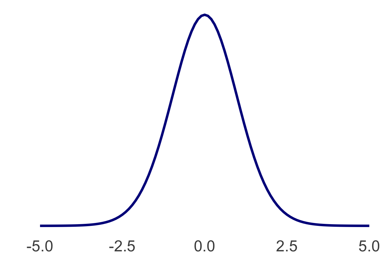
It’s almost normal—although not quite—and it has 31 degrees of freedom, a mean of 0, and a standard deviation of the \(S_M\) you just calculated.
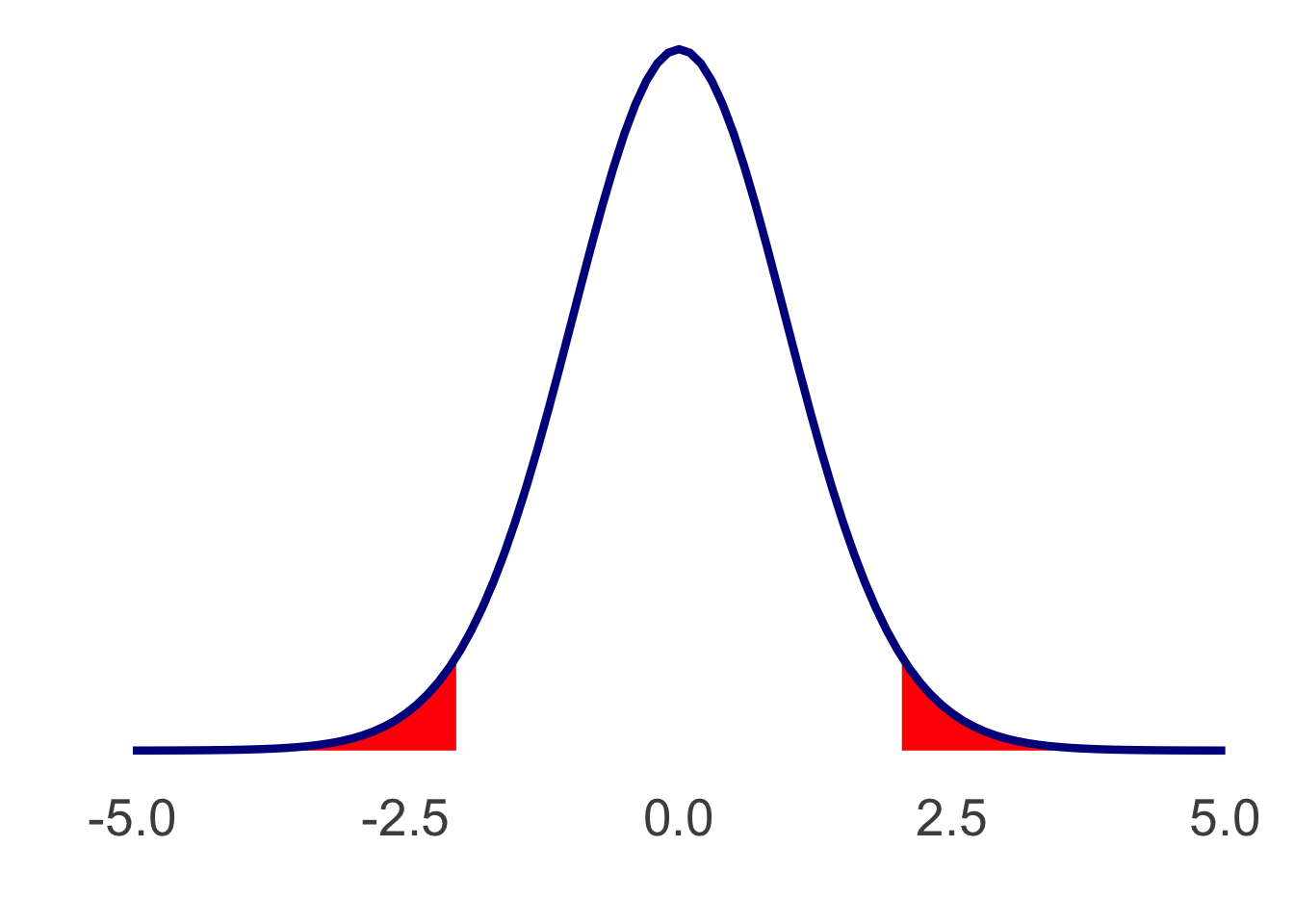
Step 3: Determine the sample cutoff score
This hasn’t changed from last time we discussed it; you could use your t-table with the degrees of freedom you found. I’ll tell you that the cutoff score is \(\pm2.04\).
This gives us a plot like the following:
Step 4: Determine the sample’s [t] score
Well, we’ve got all the pieces that go into the t equation:
\[t=\frac{M-\mu}{S_M}\]
- As #3 for today, write out the t equation with each of those variables replaced with your numbers. Then solve it and give me t.
Step 5: Determine whether to reject the null
Your eye can probably tell you whether we can reject the null. But, formally: is it larger than 2.04 or smaller than -2.04? You decide! We’ll return to this.
Do it with a function in Jamovi
So, the great thing about modern software is that we very rarely need to calculate things like this step-by-step. Instead, you can use the functions in Jamovi. You might recall that I said that the t-test for dependent means is essentially the t-test for a single sample whose population mean is 0, if you find the difference scores. Well, we do have the difference scores, in the column hrsd.diff.
In Jamovi, run a one-sample t-test on the HRSD difference scores. You don’t need to change anything, since the Test value by default is 0. Did you get something very close to the t-score you calculated? You should have.
Now, do it with the paired-samples test (Analyses -> T-Tests -> Paired Samples T-Test). Put hrsd.pre and hrsd.post into the “paired variables” box. Do you get the same value? You should!
Most of the time, we don’t actually calculate the difference scores—we run the paired samples t-test to think about the means themselves.
One thing to notice here: the degrees of freedom are based on the participants, not the number of scores. If this was an independent-samples test, we’d see \(df=62\) but because they’re matched, we only have one person’s difference scores which must be constrained.
Okay, two more things:
First, let’s describe our results.
- For #4, write up the results of your t-test. Include the means pre- and post-, and the actual test results in the format of t(df)=t-value, p < .05 (or p > .05). Replace df and t-value with the values from the test, and pick one of the options for p. Then, very briefly, explain your results. Is there a direction? Was this statistically-significant? What does it mean?
Now, in Jamovi, and under the paired samples t-test menu, click “Descriptives plots.” Then look at the following plot:
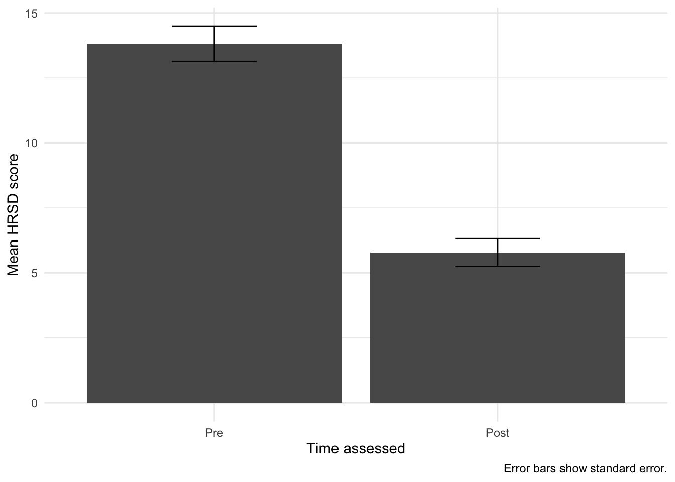
- Explain the differences between the plots. What do they tell you? Do you have a preference? This is #5.
Independent-samples t-tests
We’re not going to learn how to calculate these in the step-by-step way—that’s in the homework, but not today in lab.
But we will learn to do them with the Jamovi function.
We’re using the friends data (still here or on Brightspace).
Let’s look at the shootingdrills variable; I recoded it to have two meaningful values. We’ll have two groups here—those who had shooting drills and those who did not. But they’re not paired, so it’s an independent-samples t-test.
We can look at it relating to the numeric response asking respondents to predict whether they will vote in the 2024 election, expectedoutcome_4, where a 0 equals “definitely not” and a 100 is “100%”.
Now we want to ask this: are those who have shooting drills more likely to vote in 2024?
Do note: we started with 31 observations (respondents) here, and of those there are only 10 respondents who did not have shooting drills and 13 who did. So 8 people didn’t respond to this question. Nonetheless! We can do the test.
In Jamovi, load the friends data. Click on Analyses, T-Tests, Independent Samples T-Test. Put shootingdrills into the Grouping Variable and expectedoutcome_4 into the Dependent Variable.
- For #6: write up these results.
Okay, now do these on your own.
With the
friendsdata, use thecigarettescolumn (whether or not they’re a smoker) and thelike.dancecolumn (how much they like to dance). Is smoking a predictor of how much people like to dance? Use a t-test. Write up your results. Use the steps of hypothesis-testing if that’s helpful. The important things to turn in for #7 are the results of the test and an answer to the question.We tested the fisher data’s HRSD, but not the HARS. Did anxiety significantly decrease during treatment? Do a dependent-samples t-test to find out and report the results. No need to do it by hand—use Jamovi!—but use the steps of hypothesis-testing if that would be useful. The important thing to turn in for #8 is the comparison distribution, as well as the results of the test and a concluding sentence or two.
Check in with a classmate. Turn in the results!
Reuse
Citation
BibTeX citation:
@online{dainer-best2023,
  author = {Dainer-Best, Justin},
  title = {\_T\_-Tests for Independent and Dependent Means {(Lab} 6)},
  date = {2023-10-19},
  url = {https://faculty.bard.edu/jdainerbest/stats/labs//posts/06-t-tests},
  langid = {en}
}
For attribution, please cite this work as:
Dainer-Best, Justin. 2023. “_T_-Tests for Independent and
Dependent Means (Lab 6).” October 19, 2023. https://faculty.bard.edu/jdainerbest/stats/labs//posts/06-t-tests.