
| id | position | condition | rt |
|---|---|---|---|
| 101 | sitting | incongruent | 929.0741 |
| 101 | sitting | congruent | 888.3871 |
| 102 | sitting | incongruent | 988.1818 |
| 102 | sitting | congruent | 888.6176 |
| 103 | sitting | incongruent | 945.2174 |
| 103 | sitting | congruent | 842.6970 |
| 104 | sitting | incongruent | 913.6667 |
| 104 | sitting | congruent | 735.3125 |
| 105 | sitting | incongruent | 935.3125 |
| 105 | sitting | congruent | 818.9706 |
| 106 | sitting | incongruent | 867.1250 |
| 106 | sitting | congruent | 814.7429 |
| 107 | sitting | incongruent | 936.4000 |
| 107 | sitting | congruent | 785.2857 |
| 108 | sitting | incongruent | 764.7879 |
| 108 | sitting | congruent | 693.9429 |
| 109 | sitting | incongruent | 985.7308 |
| 109 | sitting | congruent | 961.8000 |
| 110 | sitting | incongruent | 976.2800 |
| 110 | sitting | congruent | 830.9355 |
| 112 | sitting | incongruent | 780.5588 |
| 112 | sitting | congruent | 706.3056 |
| 114 | sitting | incongruent | 950.6667 |
| 114 | sitting | congruent | 752.6471 |
| 115 | sitting | incongruent | 865.3000 |
| 115 | sitting | congruent | 702.5294 |
| 116 | sitting | incongruent | 734.6857 |
| 116 | sitting | congruent | 607.9167 |
| 117 | sitting | incongruent | 896.2258 |
| 117 | sitting | congruent | 815.1471 |
| 118 | sitting | incongruent | 854.0345 |
| 118 | sitting | congruent | 715.6875 |
| 119 | sitting | incongruent | 854.0833 |
| 119 | sitting | congruent | 797.0000 |
| 201 | standing | incongruent | 848.9412 |
| 201 | standing | congruent | 786.0571 |
| 202 | standing | incongruent | 930.9259 |
| 202 | standing | congruent | 933.1562 |
| 203 | standing | incongruent | 860.8182 |
| 203 | standing | congruent | 771.5556 |
| 204 | standing | incongruent | 895.0345 |
| 204 | standing | congruent | 767.9375 |
| 205 | standing | incongruent | 856.3333 |
| 205 | standing | congruent | 792.0000 |
| 206 | standing | incongruent | 907.2903 |
| 206 | standing | congruent | 858.3636 |
| 207 | standing | incongruent | 868.2188 |
| 207 | standing | congruent | 816.9722 |
| 208 | standing | incongruent | 780.1176 |
| 208 | standing | congruent | 682.0000 |
| 209 | standing | incongruent | 858.9706 |
| 209 | standing | congruent | 833.9394 |
| 210 | standing | incongruent | 934.1905 |
| 210 | standing | congruent | 909.6071 |
| 212 | standing | incongruent | 802.3030 |
| 212 | standing | congruent | 723.4545 |
| 214 | standing | incongruent | 883.6957 |
| 214 | standing | congruent | 804.3714 |
| 215 | standing | incongruent | 897.5312 |
| 215 | standing | congruent | 709.7647 |
| 216 | standing | incongruent | 711.2424 |
| 216 | standing | congruent | 624.0882 |
| 217 | standing | incongruent | 840.7333 |
| 217 | standing | congruent | 703.8056 |
| 218 | standing | incongruent | 901.6875 |
| 218 | standing | congruent | 807.5806 |
| 219 | standing | incongruent | 860.8421 |
| 219 | standing | congruent | 827.9600 |
Objectives
Today’s lab’s objectives are to:
- Learn about factorial ANOVA
- Learn how to conduct a factorial ANOVA in Jamovi
There’s no answer sheet for today’s lab. However, you should plan to know how to conduct a factorial ANOVA!
Factorial ANOVA
We’ll use an example via Matthew Crump for this, based on data from Rosenbaum, Mama, & Algom (2017):
Rosenbaum, D., Mama, Y., & Algom, D. (2017). Stand by your Stroop: Standing up enhances selective attention and cognitive control. Psychological Science, 28(12), 1864–1867. https://doi.org/10.1177/0956797617721270
The paper asked the kind of odd question of whether standing up vs. sitting down influenced attention. They used the Stroop task—which you may have learned about in your classes—naming words based on the color of the letters rather than their content, which is easier when the word is the same color (e.g., red—congruent) and harder when different (e.g., red—incongruent). So we have a \(2\times{}2\) design, or a two-way factorial ANOVA. Factors are position (standing vs. sitting) and condition (congruent vs. incongruent). They had participants do a congruent Stroop while sitting and then do the incongruent Stroop. They also had folks do it while standing. Throughout, they measured how long it took for people to respond (reaction time—RT).
The data from experiment 1 follows:
You should do the following:
- Download the data from here or on Brightspace, and open it in Jamovi
- Calculate the means per condition and position (using Descriptives in Jamovi), so you wind up with 4 means (sitting/congruent; sitting/incongruent; standing/congruent; standing/incongruent). (You’ll want to have rt in Variables and condition and position in “Split By”.)
- Also get Jamovi to give you the standard error of the mean, or get the standard deviation and n, and calculate SE yourself (you can look up the equation if needed)
- Put the means and SE into Google Sheets or Excel
- Make a bar (column) plot. Add the error bars. Add labels to the axes.
We are doing this much like we did in Lab 3 or the solo project. Your plot should look something like this—but do it yourself so you know how. Struggling? Keep trying, or ask for help! Here I plot without error bars, but you should add them. At minimum, you should understand what this plot is, how to create it, and why it’s useful: it’s showing our group means.
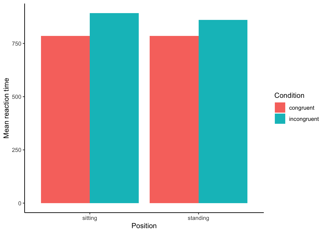
Is it clear here whether there’s a difference between conditions? We can change the y-axis to zoom in. You should be able to do the same thing in Excel or Sheets. I’m zooming to the RT between 700 and 1000ms. (I’ve also added the error bars.)
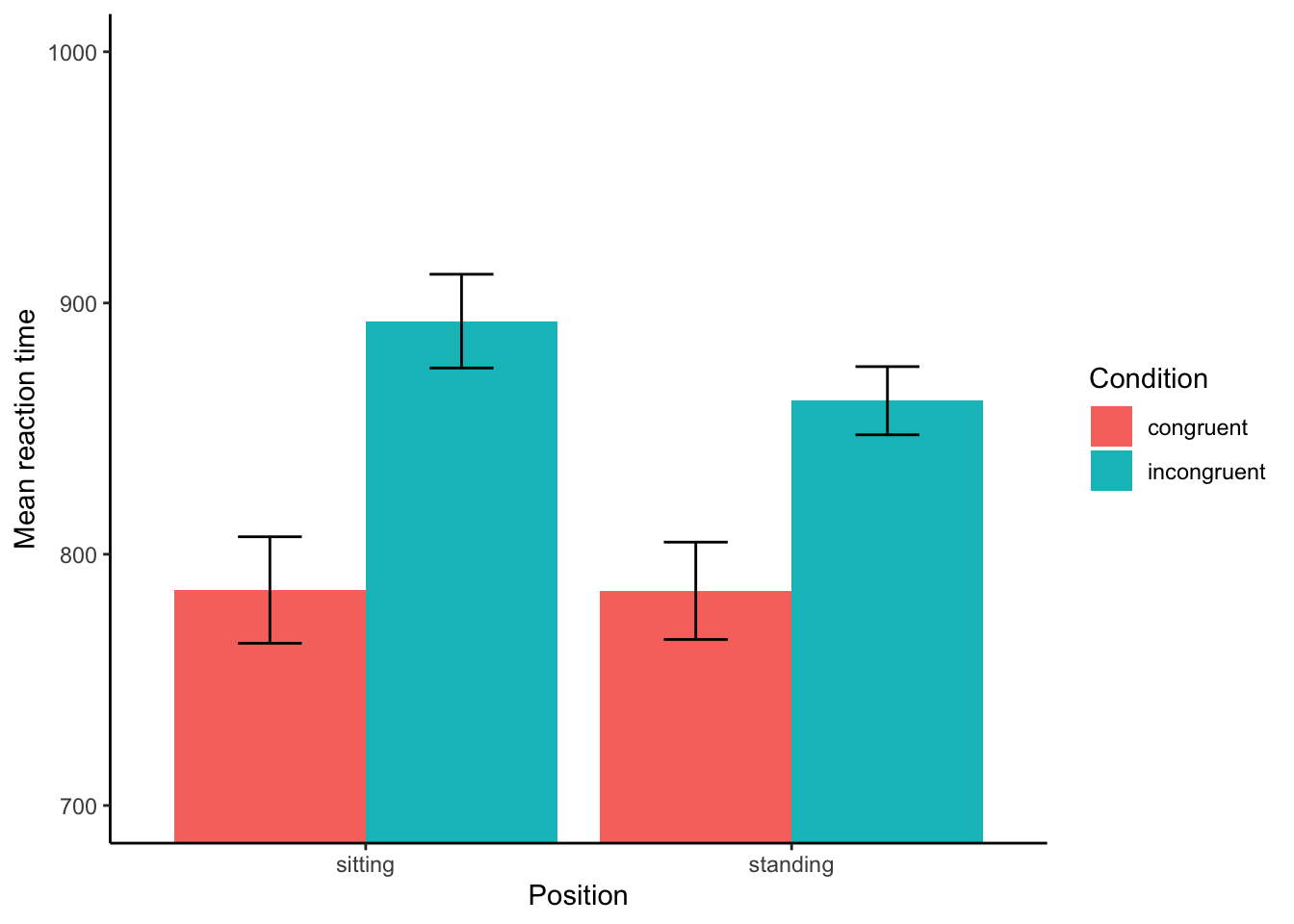
When we zoom in, it actually looks like there’s something here, perhaps? At least, there’s a main effect of condition, for sure—incongruent trials are responded to more slowly than normal. That would be a t-test, right? But is there a main effect of position? Probably not, perhaps? And is there an interaction? Well, that’s the question!
There’s more to the experiment in the original, but for us we can just conduct a factorial ANOVA.
Go to Jamovi and run the ANOVA. Put rt in the depedent variable section, and the other two terms we’re interested in (not id) in the Fixed Factors section.
Check the checkbox to also get the \(\eta^2\) (effect size). Your table should look quite similar to this:
| Sum of Squares | df | Mean Square | F | p | η2 | |
|---|---|---|---|---|---|---|
| position | 4348 | 1 | 4348 | 0.754 | 0.388 | 0.008 |
| condition | 141841 | 1 | 141841 | 24.600 | < .001 | 0.273 |
| position * condition | 4180 | 1 | 4180 | 0.725 | 0.398 | 0.008 |
| Residuals | 369011 | 64 | 5766 | — | — | — |
Spend some time trying to make sense of this. Which effects are statistically significant? Which have a meaningful effect size? Remember to start with the interaction. Then click through to confirm.
What are the conclusions from this ANOVA?
There is no significant interaction, \(F(1, 64)=0.73,p=.40\); there was no interaction between condition and prediction.
There is a main effect of condition, as we could probably tell from the plot. You can write it up using the df from above and the F and p-values: \(F(1, 64)=24.6,p<.05,\eta^2=0.27\); participants were slower to respond on incongruent trials. This effect is rather large. This implies that people responded differently in the congruent from incongruent condition. Good! We would expect to see that.
| condition | Mean RT | SD of RT |
|---|---|---|
| congruent | 785.6041 | 82.43226 |
| incongruent | 876.9473 | 68.15789 |
Yes, looks like there is a much slower reaction time (RT) to incongruent trials. They’re harder! This happens across conditions; you’ll see that if you look at your graph.
There’s no effect of position, though, \(F(1, 64)=0.75,p=.39\); participants didn’t respond more slowly when sitting or standing.
| position | Mean RT | SD of RT |
|---|---|---|
| sitting | 839.2722 | 97.57685 |
| standing | 823.2791 | 78.01138 |
And this makes sense, given that mean RT for the two positions are slightly different, but SD is large!
In Jamovi, go back to your ANOVA menu, and scroll down to “Estimated Marginal Means.” Put both condition and position in Term 1. Under Output, check the checkbox for “Marginal means plots” and “Marginal means tables.” Switch error bars to show standard error.
You should see a table that’s very similar to the one you made in Google Sheets or Excel. The means should be identical; the SE should be just about the average of what you found. They’ve also shown you 95% confidence intervals.
The plot, though, is a little different: it’s just showing the means and error bars, not a bar plot. It should look rather like this (note that if you put them in the reverse order, the plot will flip the factors; that would be fine, but will look different):
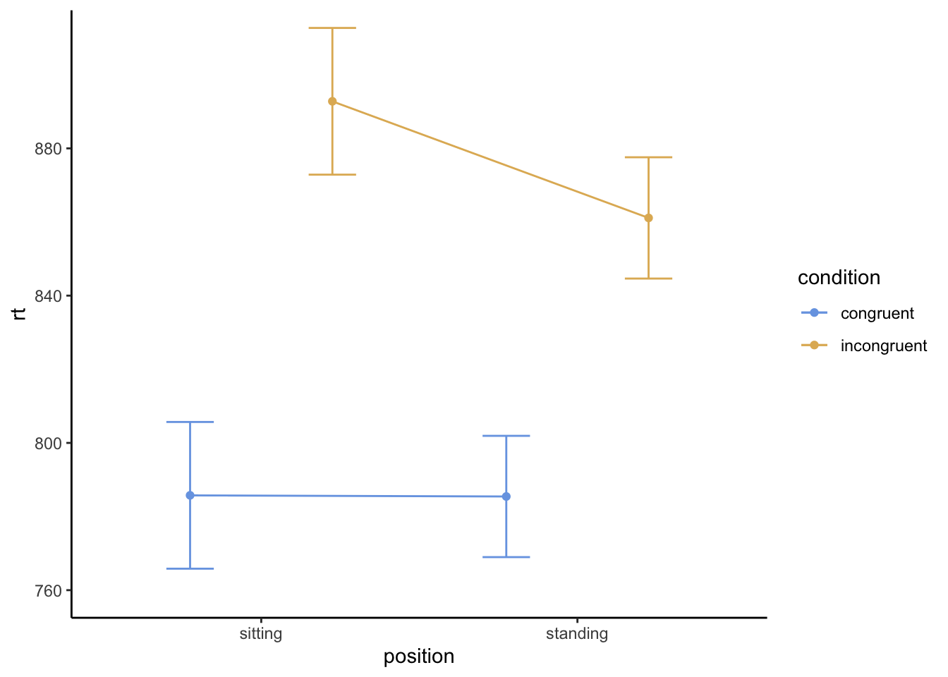
Does this plot provide different information from yours? More or less? My general sense: it’s about the same!
Interaction? What interaction?!
Because your interaction was non-significant, you could consider re-running the ANOVA without it. We’ve no real reason to suppose that we should do that here—our hypothesis involved it, I think!—but let’s learn to do it anyway. In Jamovi, scroll back up under the ANOVA to “Model”, and remove “condition * position” from the right side.
You’ll see that everything changes! The plot changes a bit (it’s using estimates from the model rather than the real data, now), and the ANOVA table looks like this:
| Sum of Squares | df | Mean Square | F | p | η2 | |
|---|---|---|---|---|---|---|
| condition | 141841 | 1 | 141841 | 24.705 | < .001 | 0.273 |
| position | 4348 | 1 | 4348 | 0.757 | 0.387 | 0.008 |
| Residuals | 373191 | 65 | 5741 | — | — | — |
What’s changed? Why do you think it has changed?
Removing the interaction means that the model changed a little bit. Since the interaction wasn’t significant—it wasn’t adding much to the model!—the values haven’t shifted much. Since the \(MS_{within}\) (under Residuals) hasn’t changed much, the \(F\) values don’t change much either. (And therefore, neither have the \(p\)s.)
The plot actually has changed more, though. This is because it’s using “estimated marginal means” based on the model, rather than the actual means we were calculating.
Assumptions Made
We also will be discussing assumptions in class. In Jamovi, you can click on “Assumption Checks” and run tests of the assumption of normality and homogeneity of variance. Re-run the model with position * condition included, then add the assumption checks.
You’ll see Levene’s test for homogeneity of variance, which we can report as \(F(3, 64)=1.39,p=.25\). If this were significant, it would mean we were violating our assumption that variance is similar between groups. Since it’s not, we can continue with this assumption.
You’ll also see the Shapiro-Wilk test for normality. Again, the p-value is non-significant (\(p=.37\)) which means that our assumption is not violated. The residuals are (relatively) normal.
In principle, as we’ll discuss, if these were significant, we’d need to make some sort of correction.
Penguins!
Let’s switch gears!
Remember that penguin data from the beginning of the semester? Go find it on Brightspace (or on your computer, or download it here), and open it in Jamovi. We’re going to ask some questions using the grouping variables.
Once you have the data open, use a Filter to ignore the penguins for whom sex is not known (i.e., set sex != NA in the filter.
Please remember that because NA is a special designation (it means “not available” here), it doesn’t have quotes. But normally it’s only the variable names, or numbers, that don’t have quotation marks. If we were only trying to filter to male penguins, we’d write sex == "male".
Use the ANOVA menu to answer whether there is an interaction between penguin sex and the island they live on in predicting body_mass_g. Then practice writing up the results. Once you’re done, click through to see my answer.
What are the conclusions from the penguin ANOVA?
| Sum of Squares | df | Mean Square | F | p | |
|---|---|---|---|---|---|
| sex | 2.71 × 10⁷ | 1 | 2.71 × 10⁷ | 95.844 | < .001 |
| island | 8.25 × 10⁷ | 2 | 4.12 × 10⁷ | 145.575 | < .001 |
| sex * island | 1.06 × 10⁶ | 2 | 5.32 × 10⁵ | 1.877 | 0.155 |
| Residuals | 9.26 × 10⁷ | 327 | 2.83 × 10⁵ | — | — |
There was no interaction between sex and island, \(F(2, 327)=1.88,p=.16\), but there was a main effect of sex, \(F(1, 327)=95.84,p<.05\) and a main effect of island, \(F(2,327)=145.58,p<.05\).
| M | SD | n | sem | |
|---|---|---|---|---|
| female | ||||
| Biscoe | 4319.38 | 659.75 | 80 | 73.76 |
| Dream | 3446.31 | 269.52 | 61 | 34.51 |
| Torgersen | 3395.83 | 259.14 | 24 | 52.90 |
| male | ||||
| Biscoe | 5104.52 | 714.20 | 83 | 78.39 |
| Dream | 3987.10 | 349.52 | 62 | 44.39 |
| Torgersen | 4034.78 | 372.47 | 23 | 77.67 |
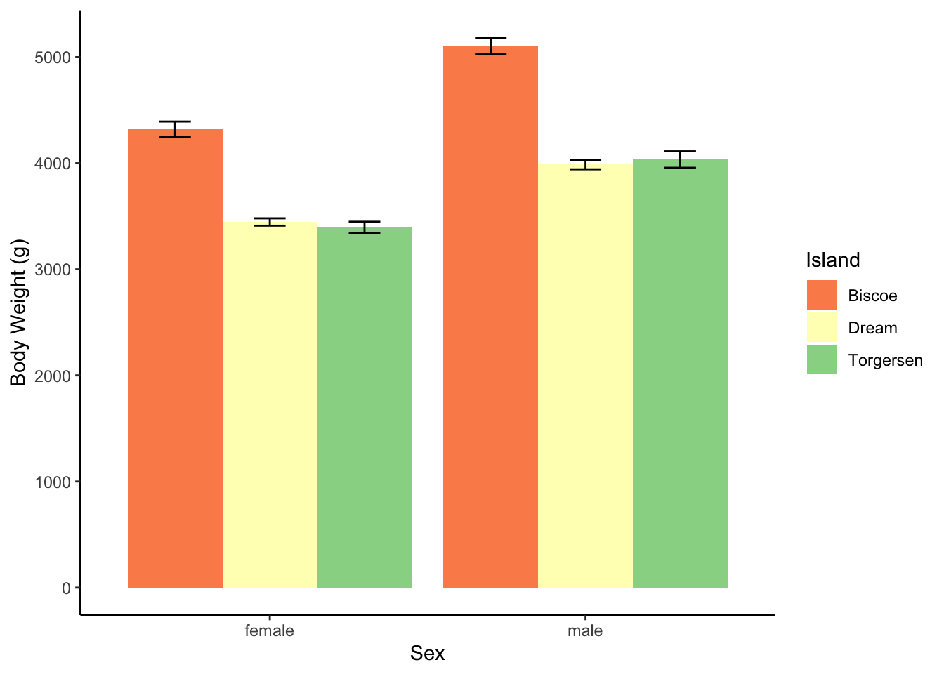
Get Jamovi to make you a plot as well. Which island has heavier penguins? Which sex is heavier?
Dream penguins only
Filter to only penguins who lives on the island Dream. (Remember to use quotation marks.) Then run an ANOVA to determine whether body_mass_g is predicted by the interaction between sex and species on Dream.
Make a plot, and try to answer the questions about which sex/species is heavier. Is there an interaction? Practice writing up the results. Once you’re done, click through to see my answer.
What are the conclusions from the second penguin ANOVA?
| Sum of Squares | df | Mean Square | F | p | |
|---|---|---|---|---|---|
| sex | 9.41 × 10⁶ | 1 | 9.41 × 10⁶ | 100.604 | < .001 |
| species | 4.41 × 10⁴ | 1 | 4.41 × 10⁴ | 0.472 | 0.494 |
| sex * species | 6.36 × 10⁵ | 1 | 6.36 × 10⁵ | 6.800 | 0.01 |
| Residuals | 1.11 × 10⁷ | 119 | 9.36 × 10⁴ | — | — |
There was an interaction between sex and species, \(F(1, 119)=6.8,p<.05\). There was also a main effect of sex, \(F(1, 119)=100.6,p<.05\). There was no main effect of species, \(F(1,119)=0.47,p=.49\). (There were only two species on the Dream island.)
| M | SD | n | sem | |
|---|---|---|---|---|
| female | ||||
| Adelie | 3344.44 | 212.06 | 27 | 40.81 |
| Chinstrap | 3527.21 | 285.33 | 34 | 48.93 |
| male | ||||
| Adelie | 4045.54 | 330.55 | 28 | 62.47 |
| Chinstrap | 3938.97 | 362.14 | 34 | 62.11 |
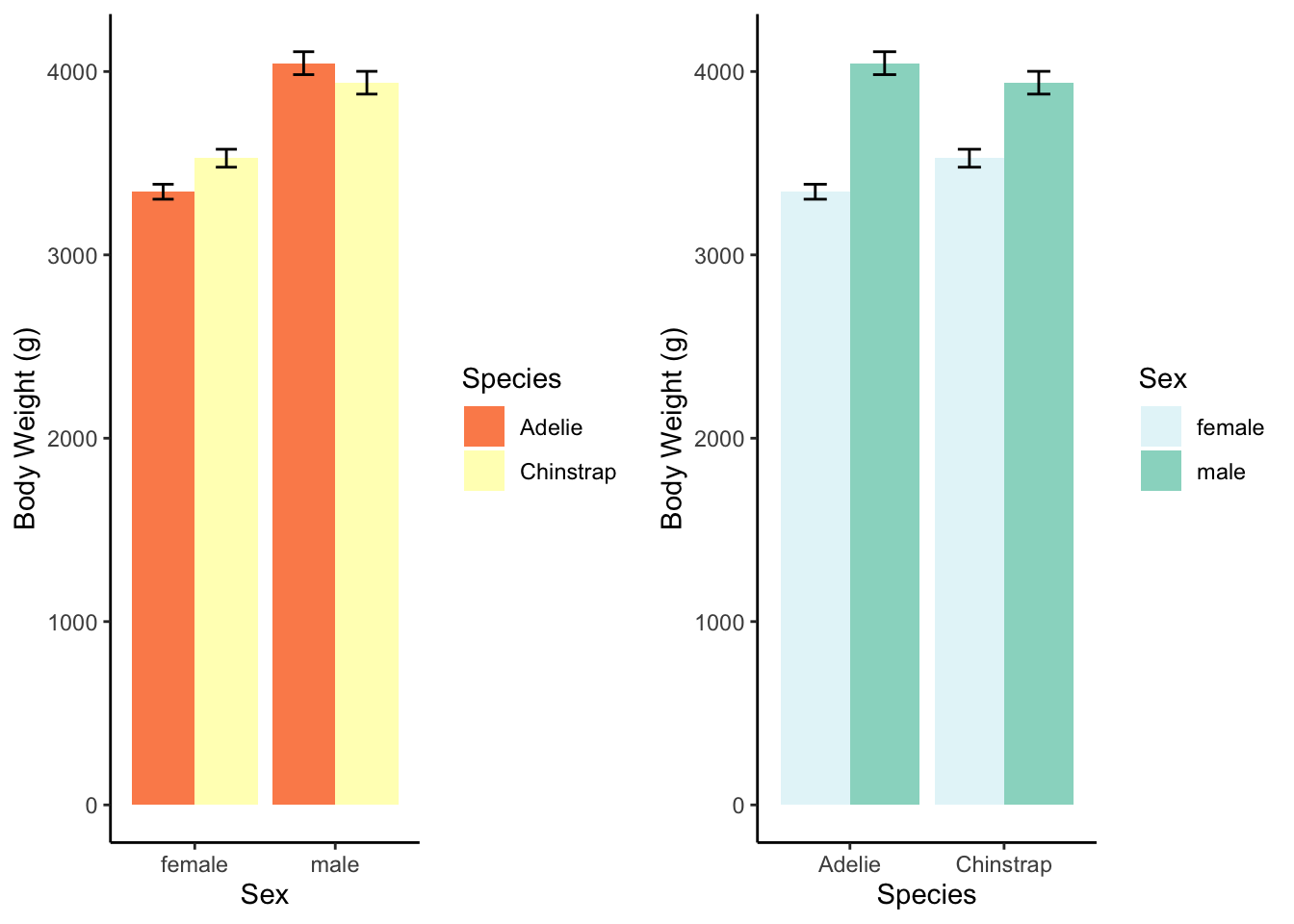
The interaction, explained: Adelie males are heavier than Chinstrap males, but Adelie females are not as heavy as Chinstrap females. But the species are roughly similar in weight.
That’s it! If you’re still finding filters or plots a challenge, or have questions about running ANOVA in Jamovi, take advantage of the stats study rooms, tutors, or my office hours.
Reuse
Citation
BibTeX citation:
@online{dainer-best2023,
  author = {Dainer-Best, Justin},
  title = {Factorial {ANOVA} {(Lab} 10)},
  date = {2023-11-16},
  url = {https://faculty.bard.edu/jdainerbest/stats/labs//posts/10-factorial-anova},
  langid = {en}
}
For attribution, please cite this work as:
Dainer-Best, Justin. 2023. “Factorial ANOVA (Lab 10).”
November 16, 2023. https://faculty.bard.edu/jdainerbest/stats/labs//posts/10-factorial-anova.