
Objectives
Today’s lab’s objectives are to:
- Learn about running chi-squared tests in Jamovi
- Do some basic plotting relating to them
You’ll turn in an “answer sheet” on Brightspace. Please turn that in by the end of the weekend.
Chi-square tests
A chi-square[d] test (\(\chi^2\)) asks whether observed frequencies fit an expected pattern. (“Observed” [what you’ve got] vs. “expected” [what you expected] frequencies.)
In the goodness of fit test, we compare how well a single nominal variable’s distribution fits an expected distribution of that variable.
In the chi-squared test of independence, we test hypotheses about the relationship between two nominal variables, comparing observed frequencies to the frequencies we would expect if there were no relationship.
The test is based on the chi-squared distribution, which we’ve discussed in class.
The distribution
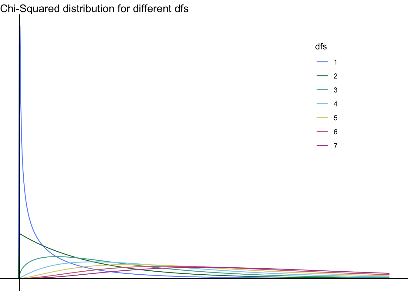
The chi-square distribution looks different at different degrees of freedom—take a look:
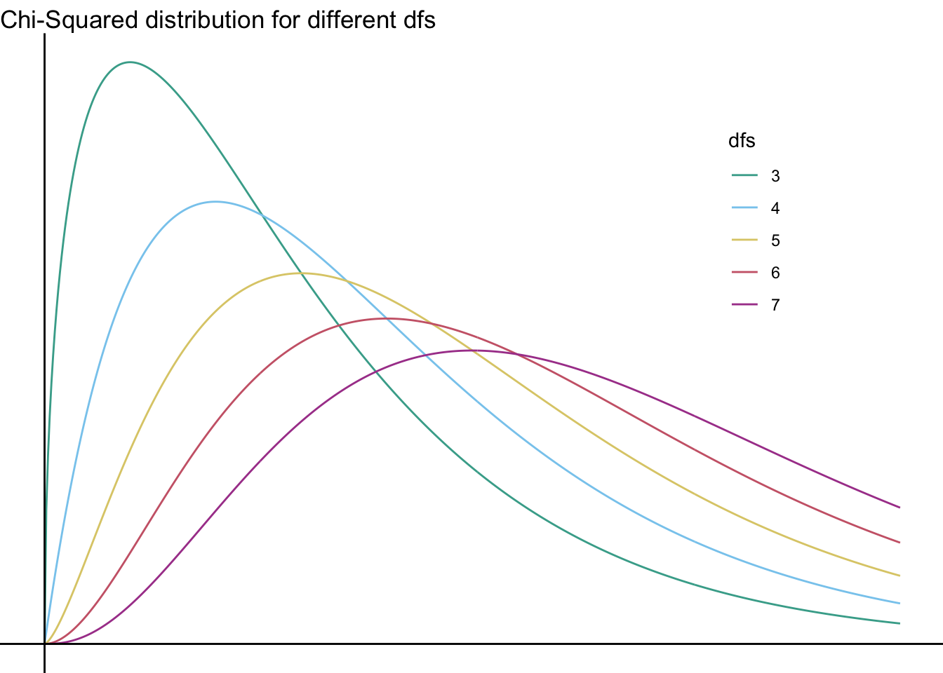
As you can see, the \(\chi^2\) distribution with \(\mathit{df}=1\) is rather different from the others; here—take a look without it:

They continue to differ even without \(\mathit{df}=2\):
As you can see, none of these distributions looks normal… you can’t (and should not!) run a useful chi-squared test with 100 categories, but if you could it would finally start to look sort of normal—just shifted to the right:
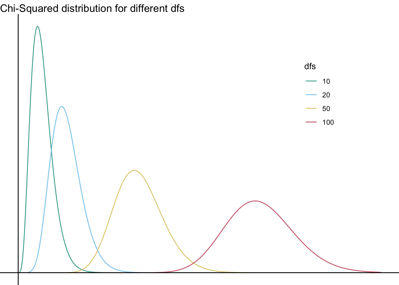
(And as we discussed in class, the cut-off for significance of that test with \(df=100\) would be… absurd. It’s very high: \(\chi^2_{crit}(100)124.3\) For comparison, recall that the cutoff for \(df=1\) is 3.84.)
Using the chi-squared test in Jamovi
The chi-squared tests in Jamovi are under the menu Frequencies.
First, the goodness of fit test
The function can help you determine whether there are the same number of participants who fall into the same boxes across conditions. (e.g., are the same number of participants selecting different gender options?)
In this kind of test, the null hypothesis is that there are the same number of participants in each group—i.e., that there are no differences between conditions. (Put another way, it’s the same percentage likelihood [probability] that any box will be chosen.) The chi-squared test for goodness of fit determines whether it is unlikely that the data comes from the null distribution.
For example, imagine that there are 100 participants who all give you the type of pet they have, and you get the following data. The null hypothesis is that (of the four pet types) there is a 25% chance that any given participant would choose them. The research hypothesis is that this is not the case—some pets are more likely to be owned by participants.
I’ve created some fake data—the below imagines that of the folks polled, 40 have cats, 55 have dogs, 3 have parakeets, and somehow 2 have pot-belly pigs:
| participant_id | pet |
|---|---|
| 1 | cats |
| 2 | cats |
| 3 | cats |
| 4 | cats |
| 5 | cats |
| 6 | cats |
| 7 | cats |
| 8 | cats |
| 9 | cats |
| 10 | cats |
| 11 | cats |
| 12 | cats |
| 13 | cats |
| 14 | cats |
| 15 | cats |
| 16 | cats |
| 17 | cats |
| 18 | cats |
| 19 | cats |
| 20 | cats |
| 21 | cats |
| 22 | cats |
| 23 | cats |
| 24 | cats |
| 25 | cats |
| 26 | cats |
| 27 | cats |
| 28 | cats |
| 29 | cats |
| 30 | cats |
| 31 | cats |
| 32 | cats |
| 33 | cats |
| 34 | cats |
| 35 | cats |
| 36 | cats |
| 37 | cats |
| 38 | cats |
| 39 | cats |
| 40 | cats |
| 41 | dogs |
| 42 | dogs |
| 43 | dogs |
| 44 | dogs |
| 45 | dogs |
| 46 | dogs |
| 47 | dogs |
| 48 | dogs |
| 49 | dogs |
| 50 | dogs |
| 51 | dogs |
| 52 | dogs |
| 53 | dogs |
| 54 | dogs |
| 55 | dogs |
| 56 | dogs |
| 57 | dogs |
| 58 | dogs |
| 59 | dogs |
| 60 | dogs |
| 61 | dogs |
| 62 | dogs |
| 63 | dogs |
| 64 | dogs |
| 65 | dogs |
| 66 | dogs |
| 67 | dogs |
| 68 | dogs |
| 69 | dogs |
| 70 | dogs |
| 71 | dogs |
| 72 | dogs |
| 73 | dogs |
| 74 | dogs |
| 75 | dogs |
| 76 | dogs |
| 77 | dogs |
| 78 | dogs |
| 79 | dogs |
| 80 | dogs |
| 81 | dogs |
| 82 | dogs |
| 83 | dogs |
| 84 | dogs |
| 85 | dogs |
| 86 | dogs |
| 87 | dogs |
| 88 | dogs |
| 89 | dogs |
| 90 | dogs |
| 91 | dogs |
| 92 | dogs |
| 93 | dogs |
| 94 | dogs |
| 95 | dogs |
| 96 | parakeets |
| 97 | parakeets |
| 98 | parakeets |
| 99 | potbellypigs |
| 100 | potbellypigs |
Now, as you see with the data above, this is just a string of animals with “id” numbers. It’s essentially nominal (categorical) data. But the chi-square test doesn’t care about participant ID at all.
If we want to run the goodness-of-fit test by hand, we need a summary table of this data. Just the counts! Something like this:
| pet | count |
|---|---|
| cats | 40 |
| dogs | 55 |
| parakeets | 3 |
| potbellypigs | 2 |
This is still nominal data. It’s just tabulated now—the numbers we’re seeing are the counts of how many people responded to each. Regardless, it sure seems like those are uneven counts. So: suppose we want to use a chi-squared test to determine whether there’s a statistically-significant difference. We can do this in two ways in Jamovi. Let’s start with that tabulated data.
In Jamovi, open a blank data set. (Close any data you have now, or go to the hamburger menu and click New.) Label one variable pet, and enter the names as you see above. Label the second variable n, or count, and enter the counts.
Then go to Analyses: Frequencies: N Outcomes (\(\chi^2\) Goodness of fit). Put pet in the Variable, and include count (or n) as the Counts. The output should be telling you: yes, there are differences in the groups! The null hypothesis can be rejected. You can write this up as follows:
There is a difference between expected and observed results in the types of pets participants had, \(\chi^2(3)=85.5, p<.05\).
Remember what I said about probabilities above? The chi-squared test determines whether it is unlikely that the data comes from a distribution of probabilities [likelihoods].
We could explicitly articulate our null hypothesis by saying that we anticipate all probabilities to be the same. Working with the same test in Jamovi, click the Expected Probabilities dropdown. Make sure the Ratio listed is 1 for all levels. (The Proportion will therefore be .25 for each.)
This is just doing the background of the chi-squared formula for you:
\[\chi^2=\sum{\frac{(O-E)^2}{E}}\]
So given the numbers of 40, 55, 3, and 2—the observed values—and the “expected” values if there were 25% response for each animal (in fact: 25, 25, 25, 25)—this is doing the calculation:
\[\chi^2=\sum{\frac{(O-E)^2}{E}}=\frac{(40-25)^2}{25}+\frac{(55-25)^2}{25}+\frac{(3-25)^2}{25}+\frac{(2-25)^2}{25}\] \[=9+36+19.36+21.16=85.52\]
… which, yes, is the same thing our test got us in Jamovi.
The interesting thing about the probabilities is that we can also suggest, e.g., that we anticipate something other than even likelihoods. For example, suppose I thought that 45% of participants would choose dogs, 45% would choose cats, 5% would choose parakeets, and 5% would have pot-bellied pigs. That’s the new null hypothesis—we are asking “are those probabilities representative of what we found?”. What does that look like in Jamovi?
Well, we just change the probabilities from 25% each to the new ones. Jamovi wants ratios; you could put them in as 45, 45, 5, 5, or as 9, 9, 1, 1 (i.e., the simplified fraction), or some other way. Try it out in Jamovi.
Are the results still statistically significant? How would you report the results?
They are no longer statistically significant. This means that now we no longer reject the null that the true counts match what we’d expect to see.
We can say that there is no difference between expected and observed results in the types of pets participants had, \(\chi^2(3)=5.3, p=.15\).
Thus, with this null hypothesis, our findings are just about what we expected! Yeah, we’d expect most people to have cats and dogs.
It might also be that case that we’d actually expect 0% pot-bellied pigs, though, even though we do live near a lot of farms. You can put in a 0 to the ratio, but it doesn’t make “sense” conceptually, even though Jamovi will give you a response.
Why doesn’t it make sense?
You divide by the expected value in the chi-square test. Dividing by 0 is not possible!
In fact, one of the assumptions of the chi-squared test is that the expected value in each cell is greater than 5. And 0% isn’t going to result in an expected value of anything other than 0!
Let’s look at another example of the chi-squared test for goodness of fit, using the penguins data again. You can still find it on Brightspace (or on your computer, or download it here), and open it in Jamovi. It might just be in your “recent data” in Jamovi.
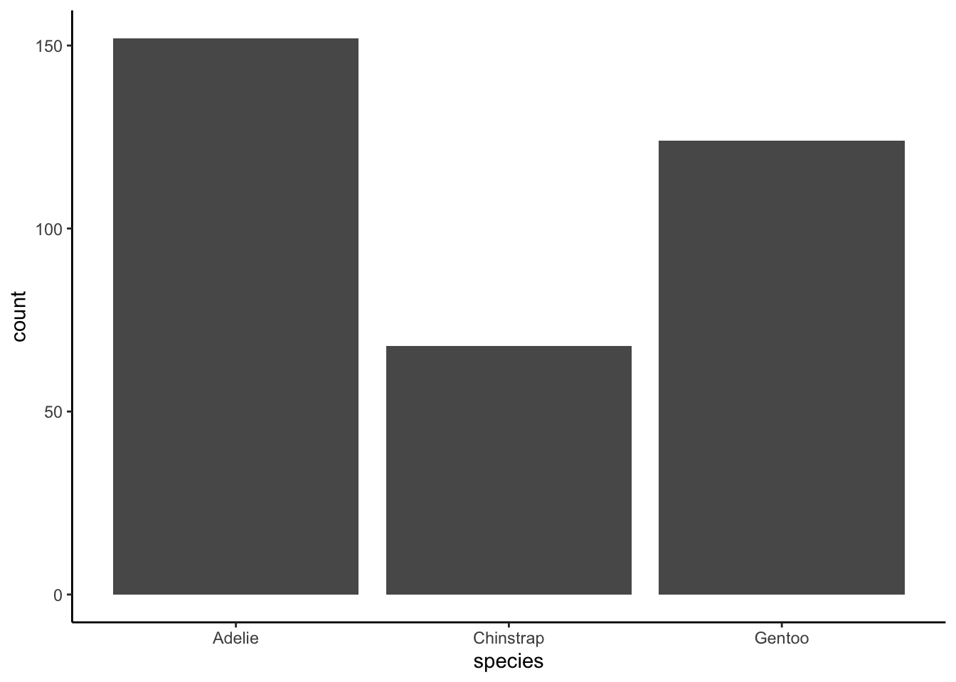
Suppose we wanted to know if the numbers of penguins of each species in the study were significantly different from one another.
| species | count |
|---|---|
| Adelie | 152 |
| Chinstrap | 68 |
| Gentoo | 124 |
Seems like a substantial difference, no? Well, is it?
This time, rather than adding the counts, just put species in the Variable field. Jamovi will automatically tabulate them for you—you should see the same numbers as above. Determine if those are different numbers per group.
Are there statistically-significant different numbers of each species?
Definitely, yes! Your results should show significant differences from the expected “even” distribution, \(\chi^2(2)=31.9, p<.05\).
As a note: you could plot these, just as you can plot any categorical data. As you may recall from the lecture on visualizations, I recommend a sorted frequency bar plot if you have more than five categories. For penguin species, it’s probably no help to sort. Something like the following would be fine:
Okay! Hopefully you’re feeling like you get what the chi-square test for goodness of fit looks like!
Let’s turn to…
Chi-square test for independence
In the test of independence, we test hypotheses about the relationship between two nominal variables, comparing observed frequencies to the frequencies we would expect if there were no relationship.
Let’s use a data-set called color:
| ColorPref | Personality |
|---|---|
| Green | Introvert |
| Green | Introvert |
| Green | Introvert |
| Green | Introvert |
| Green | Introvert |
| Green | Introvert |
| Green | Introvert |
| Green | Introvert |
| Green | Introvert |
| Green | Introvert |
| Green | Introvert |
| Green | Introvert |
| Green | Introvert |
| Green | Introvert |
| Green | Introvert |
| Green | Introvert |
| Green | Introvert |
| Green | Extravert |
| Green | Extravert |
| Green | Extravert |
| Green | Extravert |
| Green | Extravert |
| Green | Extravert |
| Yellow | Extravert |
| Yellow | Extravert |
| Yellow | Extravert |
| Yellow | Introvert |
| Yellow | Introvert |
| Yellow | Introvert |
| Yellow | Introvert |
| Yellow | Introvert |
| Yellow | Introvert |
| Yellow | Introvert |
| Yellow | Extravert |
| Yellow | Extravert |
| Red | Extravert |
| Red | Extravert |
| Red | Extravert |
| Red | Extravert |
| Red | Extravert |
| Red | Extravert |
| Red | Extravert |
| Red | Extravert |
| Red | Extravert |
| Red | Extravert |
| Red | Introvert |
| Red | Introvert |
| Red | Introvert |
| Red | Introvert |
| Red | Extravert |
Take a look above. Imagine that the “research question” is: does personality type (Personality) affect favorite color (ColorPref)?
Again, we can get a table of these—looks similar to the cells in a factorial ANOVA, huh? This is called a contingency table. It shows counts organized by cells.
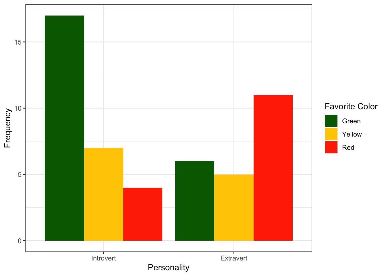
| Green | Yellow | Red | |
|---|---|---|---|
| Introvert | 17 | 7 | 4 |
| Extravert | 6 | 5 | 11 |
From this table, you should see that we might ask a question like “do introverts have a different level of liking for these colors than extraverts?” Again, what we have here are categorical variables—but we can ask a question about who falls into which category. (The numbers here are counts based on those categorical variables.)
Before we go further, let’s try plotting these cells out. Much like with a factorial ANOVA, the plot is often the best way of figuring something like this out. Looking at the plot below, do you think that there is a difference in counts between personalities in this (made up) sample? What is your hypothesis based on the plot?
Don’t worry; you can make a table quite like this in Jamovi. (You could make it in Excel or Google Sheets, too, but we’re not going to do that today… although I think you ought to know!) Copy the data from the table above (not including the header line that says ColorPref Personality). Make a new dataset in Jamovi. Paste the data in, and then label the variables ColorPref and Personality. Go to Analyses: Frequencies: Independent Samples (\(\chi^2\) test of association). Put Personality in Rows and put ColorPref in Columns. Then, scroll down to Plots and check Bar Plot.
Your plot should match this in all but color. (You can also flip the axes under where it says “X-Axis”.)
You can also enter the contingency table into Jamovi. Clear the data again (hamburger menu: New). Label your three variables Personality, ColorPref, and n. Then enter the data as follows (copy this or enter it manually):
| Personality | ColorPref | n |
|---|---|---|
| Introvert | Green | 17 |
| Introvert | Yellow | 7 |
| Introvert | Red | 4 |
| Extravert | Green | 6 |
| Extravert | Yellow | 5 |
| Extravert | Red | 11 |
You should be able to make the same plot, this time by adding the n column as your counts.
Okay, let’s look at the results of the chi-squared test. No, these are not independent variables. We can write this up as follows:
Groups were not independent—there was a link between personality and color, \(\chi^2(2)=8.26,p<.05\).
Fortunately, the mechanics of running this kind of test in Jamovi aren’t any different from running a chi-squared test of independence!
Some goodness of fit practice
Imagine that we get some data on rolling a six-sided die 150 times. You get 150 numbers between 1 and 6, representing your throwing a die over and over again. I’ve made that fake data and tabulated it for you:
| rolls | count |
|---|---|
| 1 | 39 |
| 2 | 23 |
| 3 | 18 |
| 4 | 12 |
| 5 | 19 |
| 6 | 39 |
Let’s say we want to run a chi-square test of goodness of fit on this table.
What would a p-value less than .05 mean here?
That the die is NOT fitting our expected values—we’re not seeing even choices of numbers 1-6 on this die. Maybe it’s a cheat or loaded die?
Run the chi-square test. Report the results on your answer sheet as #1.
An independence example
The data below is a “contingency table” which contains 13 house tasks and their distribution in heterosexual couples. Rows are the different tasks; values are the frequencies of the tasks done: by the wife only, by the husband only, by alternating partners, or together.
| Wife | Alternating | Husband | Jointly | |
|---|---|---|---|---|
| Laundry | 156 | 14 | 2 | 4 |
| Main_meal | 124 | 20 | 5 | 4 |
| Dinner | 77 | 11 | 7 | 13 |
| Breakfeast | 82 | 36 | 15 | 7 |
| Tidying | 53 | 11 | 1 | 57 |
| Dishes | 32 | 24 | 4 | 53 |
| Shopping | 33 | 23 | 9 | 55 |
| Official | 12 | 46 | 23 | 15 |
| Driving | 10 | 51 | 75 | 3 |
| Finances | 13 | 13 | 21 | 66 |
| Insurance | 8 | 1 | 53 | 77 |
| Repairs | 0 | 3 | 160 | 2 |
| Holidays | 0 | 1 | 6 | 153 |
| chore | who | number |
|---|---|---|
| Laundry | Wife | 156 |
| Laundry | Husband | 2 |
| Laundry | Alternating | 14 |
| Laundry | Jointly | 4 |
| Main_meal | Wife | 124 |
| Main_meal | Husband | 5 |
| Main_meal | Alternating | 20 |
| Main_meal | Jointly | 4 |
| Dinner | Wife | 77 |
| Dinner | Husband | 7 |
| Dinner | Alternating | 11 |
| Dinner | Jointly | 13 |
| Breakfeast | Wife | 82 |
| Breakfeast | Husband | 15 |
| Breakfeast | Alternating | 36 |
| Breakfeast | Jointly | 7 |
| Tidying | Wife | 53 |
| Tidying | Husband | 1 |
| Tidying | Alternating | 11 |
| Tidying | Jointly | 57 |
| Dishes | Wife | 32 |
| Dishes | Husband | 4 |
| Dishes | Alternating | 24 |
| Dishes | Jointly | 53 |
| Shopping | Wife | 33 |
| Shopping | Husband | 9 |
| Shopping | Alternating | 23 |
| Shopping | Jointly | 55 |
| Official | Wife | 12 |
| Official | Husband | 23 |
| Official | Alternating | 46 |
| Official | Jointly | 15 |
| Driving | Wife | 10 |
| Driving | Husband | 75 |
| Driving | Alternating | 51 |
| Driving | Jointly | 3 |
| Finances | Wife | 13 |
| Finances | Husband | 21 |
| Finances | Alternating | 13 |
| Finances | Jointly | 66 |
| Insurance | Wife | 8 |
| Insurance | Husband | 53 |
| Insurance | Alternating | 1 |
| Insurance | Jointly | 77 |
| Repairs | Wife | 0 |
| Repairs | Husband | 160 |
| Repairs | Alternating | 3 |
| Repairs | Jointly | 2 |
| Holidays | Wife | 0 |
| Holidays | Husband | 6 |
| Holidays | Alternating | 1 |
| Holidays | Jointly | 153 |
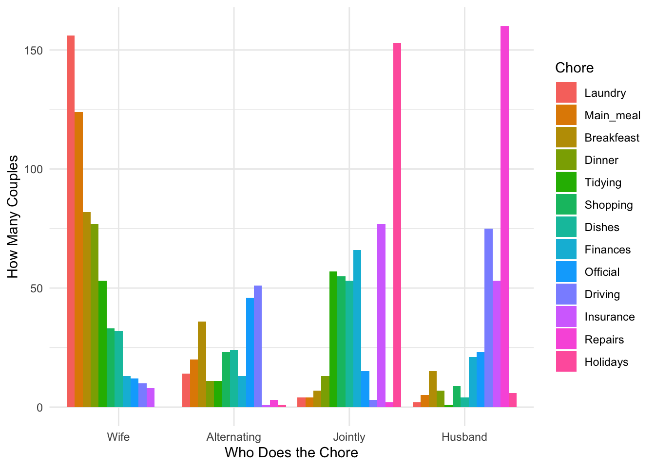
Look at the table and the plot, and make some informed guesses: in these data, are chores done evenly or unevenly?
Then use the second of the above tables (not the contingency table)—again, copy and paste into Jamovi; you may need to scroll down—to (a) recreate (as much as you can) the above graph and (b) test for independence. (This is actually a place where the stacked bar option might make sense?) Include the plot and the results as #2 on your answer sheet.
That’s the end of the lab! Feel free to meet with your group for the group project.
Reuse
Citation
BibTeX citation:
@online{dainer-best2023,
  author = {Dainer-Best, Justin},
  title = {Chi-Square {(Lab} 11)},
  date = {2023-12-07},
  url = {https://faculty.bard.edu/jdainerbest/stats/labs//posts/11-chi-square},
  langid = {en}
}
For attribution, please cite this work as:
Dainer-Best, Justin. 2023. “Chi-Square (Lab 11).” December
7, 2023. https://faculty.bard.edu/jdainerbest/stats/labs//posts/11-chi-square.